R for spatial data wrangling: using sf to wrangle pharmacies in Atlanta and assess population living nearby (Part 1)
Michael D. Garber, PhD MPH
2022-08-23
1 Objective and background
Overall goal: Illustrate use of sf through example analyses with spatially referenced pharmacy data downloaded from OpenStreetMap via osmdata and spatially referenced census data in the Atlanta area downloaded via tidycensus.
Specifically:
According to OpenStreetMap, how many pharmacies are there in Fulton and Dekalb counties (Atlanta area)?
How many people live within 1/2 mile of these pharmacies in these counties?
In part 1, we answer the first question. In part 2, we answer the second.
Background
sf object types: https://r-spatial.github.io/sf/articles/sf1.html
point
linestring
polygon
multipoint
multilinestring
multipolygon
geometry collection - set of geomtries of any type
I’d suggest reviewing these vignettes from the sf home page:
And sf is covered in these two chapters of Geocomputation with R:
Miscellaneous methods used and things to note:
Note that dplyr and sf functions can be used in the same pipe.
sf is “sticky”, meaning the geometry column “sticks around” unless you explicitly remove it, e.g., using
st_set_geometry(NULL). For example, even if you usedplyr::select()and don’t include geometry as one of the columns to select, the geometry column will remain.Illustrate use of the
st_area()function to measure area.Illustrate use of
st_union(), which smushes together multiple sf features into one single feature.Similarly, we can dissolve (ArcGIS word) census tracts into counties using the
group_by()andsummarise()syntax from dplyr.Illustrate use of
st_intersection(), which returns the geometry covered by overlapping features.Illustrate use of
st_join(), which allows for a spatial left join.Illustrate use of
st_centroid(), which finds the centroid (weighted average middle) of an sf object.Illustrate use of
st_buffer()to create a buffer area around a polygon.Illustrate use of
ggplot2()to map sf objects.
1.1 Install and load packages
#Packages needed for downloading data
install.packages("osmdata")
install.packages("tidycensus")
#Other packages used
install.packages("tidyverse") #always :)
install.packages("sf") #focus of session; spatial data wrangling
install.packages("mapview") #interactive mapping
install.packages("viridis") #for color scales.
install.packages("here") #working-directory managementlibrary(osmdata)
library(tidycensus)
library(tidyverse)
library(sf)
library(mapview)
library(viridis)
library(here)2 Download, prepare, and visualize census tract data for Georgia
Packages used in this section (besides dplyr and sf):
tidycensus to download American Community Survey data
ggplot2 to make static maps
This code chunk tells tidycensus to save the geometry locally, which can speed up the process if you end up downloading it multiple times.
options(tigris_use_cache = TRUE) Load population data for all of Georgia’s census tracts based on American Community Survey estimates (2016-2020 5-year). Recall, we can search variable names using by:
vars_acs_2020 = tidycensus::load_variables(2020, "acs5", cache = TRUE)
View(vars_acs_2019) 2.1 Download data using get_acs()
Some notes this function call:
We’re downloading, at the census-tract level:
Total population
Median home value
Median household income
Use
output="wide"so the resulting data is wide-form. It is otherwise long-form by default. This way, variable names will appear as columns and are easier to manage.I add an underscore at the end of the variable names, e.g.,
pop_,h_val_med_, because suffixes of E for estimate and M for margin of error are automatically added during theget_acs()function call. The addition of the underscore allows these suffixes to be more easily seen.
tract_ga =tidycensus::get_acs(
year=2020,
output = "wide",
geography = "tract",
state ="GA",
geometry = TRUE,
variables = c(
pop_ = "B01001_001",
h_val_med_ = "B25077_001",
hh_inc_med_ = "B19013_001")
)2.2 Wrangle data using dplyr and sf functions, including st_area(), st_transform()
Here are our first sf functions. We measure the area of each census tract using sf::st_area(), and we go back and forth between coordinate reference systems (CRS) using sf::st_transform(). I typically use WGS84, a commonly used CRS, which has the EPSG code of 4326. The main practical consideration in deciding which CRS to use is its unit of measurement (i.e., meters or feet).
Overview resources on coordinate reference systems:
List of coordinate reference systems:
https://www.spatialreference.org/ref - “bad gateway” - hopefully that resolves, as this page has a nice list of EPSG codes with output units (feet or meters)
Other topics in this code chunk:
FIPS codes:
stringr::str_sub()to extract a string by position.
tract_ga_wrangle = tract_ga %>%
dplyr::rename(
geo_id= GEOID,
name_tract_county = NAME,
pop = pop_E #simplify
) %>%
sf::st_transform(4326) %>% #
dplyr::mutate(
#Extract county 5-digit FIPS code
#first 2 digits of the FIPS code
#correspond to state. Then the next 3 indicate the county.
# Note Fulton is 13121
# Dekalb is 13089
county_fips = stringr::str_sub(geo_id, start=1, 5),
area_4326 = sf::st_area(geometry), #returns area of type "units".
#measured in meters squared because of the coordinate system.
area_m2 = as.numeric(area_4326), #convert to numeric. strip units
#indicator for major Atlanta Metro Counties
atlanta_metro = case_when(
#character format even though they're numbers, so quote
county_fips %in% c(
"13121",#fulton
"13089",#dekalb
"13135",#gwinnett
"13067", #cobb
"13063", #clayton
"13097" #douglas
) ~1,
TRUE ~0)
) %>%
#Convert it to a coordinate system that will output in feet as well.
#NAD83 / Georgia West (ftUS)
sf::st_transform(2240) %>%
dplyr::mutate(
area_2240 = sf::st_area(geometry), #square feet
area_ft2 = as.numeric(area_2240),
area_mi2 = area_ft2/27878400, #convert to square miles
#calculate population density
pop_dens_per_mi2 = pop/area_mi2
) %>%
#Remove the margins of error
dplyr::select(-ends_with("_M")) Note that we could have included the above code as part of the one above it (i.e., where tract_ga was created) all in one pipe. That would have made the code a bit more concise. When downloading from an external source, though, it can be better to limit the number of times the you call on the external source, both for computing speed (it can take a while) and because some sources (e.g., OpenStreetMap) have limits on the number of times you can download in a short period of time, as it strains their resources. So, in this case, assuming we may have to re-run the wrangling steps a few times before we’ve made our final decision, we prioritize courtesy over brevity.
Take a look at the data:
variable names:
names(tract_ga_wrangle)## [1] "geo_id" "name_tract_county" "pop"
## [4] "h_val_med_E" "hh_inc_med_E" "county_fips"
## [7] "area_4326" "area_m2" "atlanta_metro"
## [10] "area_2240" "area_ft2" "area_mi2"
## [13] "pop_dens_per_mi2" "geometry"Note units of the area measurements
class(tract_ga_wrangle$area_4326) #note units## [1] "units"class(tract_ga_wrangle$area_m2) #numeric## [1] "numeric"class(tract_ga_wrangle$area_2240) #units## [1] "units"class(tract_ga_wrangle$area_ft) #numeric## [1] "numeric"Examine household income and median home value seem using base::summary().
Median household income of census tracts
summary(tract_ga_wrangle$hh_inc_med_E)## Min. 1st Qu. Median Mean 3rd Qu. Max. NA's
## 7708 43155 58241 66021 80396 250001 33Median home value of census tracts
summary(tract_ga_wrangle$h_val_med)## Min. 1st Qu. Median Mean 3rd Qu. Max. NA's
## 9999 118800 167700 205576 250600 1276800 892.2.1 Save ACS data for use in later code
setwd(here("data-processed"))
save(tract_ga_wrangle, file = "tract_ga_wrangle.RData")2.3 Map census tracts using ggplot
2.3.1 Visualize population
Use the viridis palette, which is built into ggplot2:
https://cran.r-project.org/web/packages/viridis/vignettes/intro-to-viridis.html
https://ggplot2.tidyverse.org/reference/scale_viridis.html
Note ggplot2::scale_fill_viridis_b() automatically discretizes (breaks into groups) the color scale. The _b stands for bin for binning continuous data before the mapping.
tract_ga_wrangle %>%
ggplot2::ggplot(aes(fill = pop, color = pop))+
ggplot2::geom_sf()+
ggplot2::scale_fill_viridis_b()+ #fill color of the polygons
ggplot2::scale_colour_viridis_b() #line (border) color of the polygons
2.3.2 Visualize population density
Here I’d like to keep the scale in continuous form rather than in bins, as above, so I’m going to use the palettes directly from viridis.
tract_ga_wrangle %>%
ggplot2::ggplot(aes(fill = pop_dens_per_mi2, color = pop_dens_per_mi2))+
ggplot2::geom_sf()+
#easier to see with a continuous scale rather than the breaks
viridis::scale_fill_viridis() +
viridis::scale_color_viridis()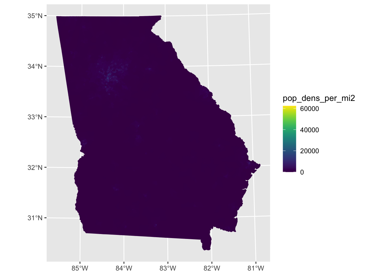
Try filtering to Atlanta Metro Counties and removing very high-population-dense census tracts, which are skewing the scale. The scale rises linearly, but the vast majority of census tracts have low density, and a few have high density, as the histogram shows:
tract_ga_wrangle %>%
ggplot2::ggplot(aes(pop_dens_per_mi2))+
geom_histogram()
tract_ga_wrangle %>%
filter(atlanta_metro==1) %>%
filter(pop_dens_per_mi2 <25000) %>%
ggplot2::ggplot(aes(fill = pop_dens_per_mi2, color = pop_dens_per_mi2))+
ggplot2::geom_sf()+
viridis::scale_fill_viridis() +
viridis::scale_color_viridis()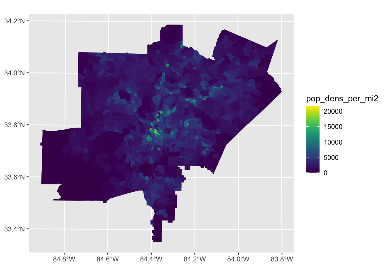
What about a different viridis color palette? And a nicer label for the legend? And can we make the coordinates look better?
Reference: http://www.cookbook-r.com/Graphs/Legends_(ggplot2)/
tract_ga_wrangle %>%
filter(atlanta_metro==1) %>%
filter(pop_dens_per_mi2 <25000) %>%
ggplot2::ggplot(aes(fill = pop_dens_per_mi2, color = pop_dens_per_mi2))+
ggplot2::geom_sf()+
#Write the same name in both, and it won't repeat.
#\n for line break (carriage return)
viridis::scale_fill_viridis(
option="magma",
name = "Pop. density \n(people per square mile)") +
viridis::scale_color_viridis(
option="magma",
name = "Pop. density \n(people per square mile)"
) +
theme_minimal()
2.4 Summarize by county to create an sf object of counties
Here, we summarize over county and keep geometry of counties. The “features” of the sf object will become counties rather than census tracts. This procedure is like a “dissolve” in ArcGIS.
county_ga = tract_ga_wrangle %>%
dplyr::group_by(county_fips) %>%
#any summary operation (e.g., average, standard deviation) will do to collapse the geometry. sum makes sense here.
dplyr::summarise(pop= sum(pop, na.rm=TRUE)) %>%
dplyr::ungroup() %>% #so we're no longer doing grouped operations
sf::st_transform(2240) %>%
dplyr::mutate(
#Measure the area of each county
area_2240 = st_area(geometry),
area_ft2 = as.numeric(area_2240),
area_mi2 = area_ft2/27878400, #convert to square miles
pop_dens_per_mi2 = pop/area_mi2 #calculate population density
) 2.5 Map census tracts using ggplot
Now, rather than keeping the lines and the fill the same color, I’m coloring the lines white so that they stand out more.
2.5.1 Visualize population
I’m using the continuous palette.
county_ga %>%
ggplot2::ggplot(aes(fill = pop))+
ggplot2::geom_sf(color = "white")+
viridis::scale_fill_viridis(name = "Population")
2.5.2 Visualize population density
#Visualize population density
county_ga %>%
ggplot(aes(fill = pop_dens_per_mi2))+
geom_sf(color = "white")+
viridis::scale_fill_viridis(
option="magma",
name = "Pop. density \n(people per square mile)" ) +
theme_minimal()
3 Download and manipulate pharmacies in Fulton and Dekalb Counties
Key packages and functions used:
osmdata to download pharmacies from OpenStreetMap
mapview
sf functions used
st_union(): unify several features into one.st_as_sf(): convert an object that is not of class sf to sf.st_buffer(): create a buffer around the features in the sf object.st_bbox(): create a bounding box (four vertices representing the min and max longitude and latitude of the sf object)st_intersection(): return the overlapping geometry of two features.st_transform(): change the coordinate reference system of an sf objectst_crs(): return the coordinate reference system of an object.st_join(): join two simple features based on whether their geometries overlap (spatial join).st_centroid(): find the weighted-average middle (centroid) of a polygon. This will convert the sf object from a polygon or multipolygon to a point.
the usual dplyr verbs and some new ones:
bind_cols()binds two or more dataframes or sf objects beside one another (adding width to data).Rows are matched by position.
The binding datasets must have the same number of rows. It differs from mutating joins like
left_join()in that you don’t need to match columns on a key.
bind_rows()stacks two or more dataframes or sf objects on top of one another (adding length to the data)Columns are matched by name.
Any columns that appear in one dataset but not the other are filled with NA.
The eventual goal is to gather a dataset of all pharmacies in Fulton County and Dekalb County. The osmdata package takes a bounding box to define the area for which to download data.
First, download all pharmacies in the bounding box defined by the min and max coordintes of Fulton and Dekalb Counties, and then restrict to the actual county boundaries.
Let’s first take a look at those counties using mapview:
Fulton is 13121
Dekalb is 13089
county_ga %>%
dplyr::filter(county_fips == "13121" | county_fips == "13089") %>%
mapview::mapview()Okay, in creating the bounding box, Fulton has the westernmost, northernmost, and southernmost coordinates, and Dekalb has the easternmost point. We could approximate the coordinates manually by clicking in Google Maps (maybe easier) or extract the coordinates with some sf functions, which could then generalize to other settings.
3.1 Use st_union() to generate a geometry file for the smashed together version of Fulton and Dekalb counties
Before we do that, let’s get smash the two counties together into one single feature.
fulton_dekalb_union = county_ga %>%
dplyr::filter(county_fips == "13121" | county_fips == "13089") %>%
sf::st_union() %>% #combine the two features into one.
sf::st_as_sf() %>% #confirm it's an sf object again.
sf::st_transform(4326) #be explicit about the coordinate system. step not necessary.Let’s take a look using mapview.
Note that several mapview layers can be combined using plus signs
Reference: https://r-spatial.github.io/mapview/articles/mapview_02-advanced.html
This situation may be one of the few where the piped style is less useful.
#Create sf objects of just Fulton County and of just Dekalb County
fulton = county_ga %>%
dplyr::filter(county_fips == "13121")
dekalb = county_ga %>%
dplyr::filter(county_fips == "13089")
#Combine multiple mapviews
mapview(fulton, col.regions = "yellow")+
mapview(dekalb, col.regions = "blue") +
mapview(fulton_dekalb_union, col.regions = "gray50") 3.2 Use st_bbox() to get the bounding box of the Fulton-Dekalb sf object
bbox_fulton_dekalb = fulton_dekalb_union %>%
sf::st_bbox() #returns the bounding box of this sf objectVisualize the bounding box. I’m doing some data prep beforehand to convert the bounding box, which is a list of values, back to an sf object. I use the st_as_sf() function and define the coordinates for the four points of the box as columns, respectively, of longitude and latitude. And I define the coordinate reference system as 4326 per usual.
bbox_lon = c(bbox_fulton_dekalb$xmax,
bbox_fulton_dekalb$xmin,
bbox_fulton_dekalb$xmax,
bbox_fulton_dekalb$xmin) %>%
dplyr::as_tibble() %>%
dplyr::rename(lon = value)
bbox_lat = c(bbox_fulton_dekalb$ymax, bbox_fulton_dekalb$ymax,
bbox_fulton_dekalb$ymin, bbox_fulton_dekalb$ymin) %>%
dplyr::as_tibble() %>%
dplyr::rename(lat = value)
bbox_fulton_dekalb_sf = bbox_lat %>%
dplyr::bind_cols(bbox_lon) %>% #add these columns to bbox_lat
sf::st_as_sf(coords = c("lon", "lat"), crs = 4326)
mapview(fulton_dekalb_union, col.regions = "gray50") +
mapview(bbox_fulton_dekalb_sf)## Warning in cbind(`Feature ID` = fid, mat): number of rows of result is not a
## multiple of vector length (arg 1)3.3 Use osmdata to download pharmacies in the bounding box
References:
overview of package and workflow: https://cran.r-project.org/web/packages/osmdata/vignettes/osmdata.html
Details on the
opq()function, specifically: https://www.rdocumentation.org/packages/osmdata/versions/0.1.5/topics/opqopq stands fro overpass query. Overpass is the name of the API used.
As mentioned above, the opq() function takes a bounding box to know what catchment area to download data from. The bbox argument can either be a string of maximal and minimal latitudes for the bounding box, or it can be the name of a place, from which a bounding box will be derived. For example, we could say: bbox = "Georgia, USA" .
The bounding box will be a rectangle based on the farthest apart corners. So we know exactly what we’re getting, let’s use the values from the bounding box created above. The order it expects is c(xmin, ymin, xmax, ymax).
And the “key” and “value” correspond to the data structure of OpenStreetMap.
Finally, we use osmdata::osmdata_sf() to return sf objects.
pharm= osmdata::opq (
bbox = c(
bbox_fulton_dekalb$xmin,
bbox_fulton_dekalb$ymin,
bbox_fulton_dekalb$xmax,
bbox_fulton_dekalb$ymax)
) %>%
osmdata::add_osm_feature(
key = "amenity",
value = "pharmacy") %>%
osmdata::osmdata_sf() #return an sf object3.3.1 Load the data from a local folder in case osmdata::opq() did not work.
Every now and then, this function throws an error. If this function did not work, please download the .RData file from this Dropbox folder so that you can run the rest of the code. You would then load it into your R environment using something like this, depending on the folder from which you load the data.
library(here)
#The name of your folder with the data.
setwd(here("data-input"))
load("pharm.RData")The result of this is an object of class osmdata, which is a special type of list comprised of elements containing the various types of geometry (points, polygons, etc.).
Reference: https://cran.r-project.org/web/packages/osmdata/vignettes/osmdata.html#3_The_osmdata_object
Because we used the osmdata_sf() function, each element in the list is an sf object.
Let’s take a look.
pharm## Object of class 'osmdata' with:
## $bbox : 33.502511,-84.850713,34.186289,-84.023713
## $overpass_call : The call submitted to the overpass API
## $meta : metadata including timestamp and version numbers
## $osm_points : 'sf' Simple Features Collection with 882 points
## $osm_lines : NULL
## $osm_polygons : 'sf' Simple Features Collection with 95 polygons
## $osm_multilines : NULL
## $osm_multipolygons : 'sf' Simple Features Collection with 1 multipolygonsLet’s now grab the individual sf objects from the list:
pharm_points = pharm$osm_points
pharm_polygons = pharm$osm_points
pharm_multipolygons = pharm$osm_multipolygonsNote, for reference that this could also be done using a pipe, which could be useful if we wanted to incorporate this as a part of a workflow with multiple steps. The . is a stand in for the object because $ an operator and not a function.
pharm_points = pharm %>%
.$osm_points3.3.2 Visualize the osmdata sf objects using mapview
I’m saving mapview objects so I can them layer them together.
(Note: unfortunately, a bug in mapview is mis-assigning the colors in the R Markdown html output…the colors work for me in the output from an R script.)
mv_points = pharm_points %>%
dplyr::select(osm_id, name, geometry) %>% #restrict data for parsimony
mapview(
layer.name = "points",
col.regions = "red",
color = "red")
mv_polygons = pharm_polygons %>%
dplyr::select(osm_id, name, geometry) %>%
mapview(
layer.name = "polygons",
color = "blue",
col.regions = "blue")
#This is at North and Piedmont.
mv_multipolygons = pharm_multipolygons %>%
dplyr::select(osm_id, name, geometry) %>%
mapview(
layer.name = "multipolygons",
color = "purple",
col.regions = "purple")
#Compare with the bounding box and the Fulton-Dekalb county boundaries
mv_fulton_dekalb_union = fulton_dekalb_union %>%
mapview(
layer.name = "fulton_dekalb_union",
col.regions = "gray50")
mv_bbox = bbox_fulton_dekalb_sf %>%
mapview(
layer.name = "bounding box",
col.regions = "orange",
color = "orange")## Warning in cbind(`Feature ID` = fid, mat): number of rows of result is not a
## multiple of vector length (arg 1)#Visualize all of the layerss
mv_points + mv_polygons+mv_multipolygons+
mv_fulton_dekalb_union+
mv_bboxConclusion on how to handle pharmacies represented as points vs polygons vs multipolygons: after browsing around in mapview, many of the points are simply vertices of buildings which are coded as polygons. Where this is the case, let’s remove the points and keep the polygons.
There is also one coded as multipolygon. It contains much of the metadata about the pharmacy (osm_id = 11918050), which is at North and Piedmont. So for that one, let’s keep the multipolygon and remove the polygon.
3.4 Restrict to the pharmacies in Fulton and Dekalb county
Use st_intersection(). Note this requires sf objects to be in the same coordinate system. Check that first. They’re both 4326.
sf::st_crs(pharm_points)
sf::st_crs(fulton_dekalb_union)3.4.1 st_intersection() with points
Return the intersection between the points and the unioned Fulton and Dekalb counties.
pharm_points_fd = pharm_points %>% #fd for Fulton and Dekalb.
sf::st_intersection(fulton_dekalb_union) %>%
dplyr::mutate(
type_point = 1, #indicator for point
point_row_number = row_number()) # an identifier## Warning: attribute variables are assumed to be spatially constant throughout all
## geometriesCheck the st_intersection(). Are all points inside the polygon?
mv_points_fd = pharm_points_fd %>%
mapview(
layer.name = "Points - in FD boundaries",
col.regions = "orange",
color = "orange")
mapview(fulton_dekalb_union, col.regions = "gray50") +
mv_points +
mv_points_fdCan also check by examining the number of rows in the original dataset of points and the new one that’s restricted to the county boundaries:
nrow(pharm_points_fd)## [1] 323nrow(pharm_points)## [1] 8823.4.2 st_intersection() with polygons
Return the intersection between the polygons and the unioned Fulton and Dekalb counties.
pharm_polygons_fd = pharm_polygons %>%
sf::st_intersection(fulton_dekalb_union) %>%
dplyr::mutate(
type_polygon = 1, #indicator for the forthcoming spatial join
polygon_row_number = row_number())## Warning: attribute variables are assumed to be spatially constant throughout all
## geometries3.4.3 st_intersection() with the 1 multipolygon
We know the one multipolygon is in Fulton County based on our data exploration, but run the code anyway to be consistent and future proof.
pharm_multipolygons_fd = pharm_multipolygons %>%
sf::st_make_valid() %>%
st_buffer(0) %>% #a trick if there's invalid geometry (loops)
sf::st_intersection(fulton_dekalb_union) %>%
mutate(type_multipolygon=1)## Warning: attribute variables are assumed to be spatially constant throughout all
## geometriesHow many do we have of each type within the county boundaries?
nrow(pharm_points_fd)## [1] 323nrow(pharm_polygons_fd)## [1] 323nrow(pharm_multipolygons_fd)## [1] 14 Combine the three types into a single dataset.
The goal here is to create a single dataset of pharmacies without duplicate features. These steps are preparing for a spatial join of the three feature types using st_join()
As we discovered, many of the points are simply vertices of buildings which are coded as polygons. Where this is the case, remove the points and keep the polygons. And keep the one multipolygon as well.
4.1 Use st_buffer() to make points bigger to be sure intersections are detected.
Before finding intersections, make sure the points are large enough to overlap the polygons (i.e., no false negatives). This may not be necessary here but is good insurance. Note the coordinate system is 4326, so the buffer units are meters.
In addition, in this step, I’m removing extraneous variable names using dplyr::select(). st_intersection() is like a join and will link all variables from each of the joining datasets. If the same variable name exists in both, it may cause issues.
pharm_points_fd_buff_20m = pharm_points_fd %>%
st_buffer(20) %>% #create a 20 m buffer around each point.
#keep this but rename it so it doesn't create a duplicate variable name upon linking
rename(osm_id_point = osm_id) %>%
dplyr::select(osm_id_point, type_point, point_row_number, geometry)Confirm same number of rows (i.e., no new rows added or subtracted due to buffer). And was it converted from a point to a polygon?
nrow(pharm_points_fd_buff_20m)## [1] 323nrow(pharm_points_fd)## [1] 323class(pharm_points_fd_buff_20m$geometry)## [1] "sfc_POLYGON" "sfc"class(pharm_points_fd$geometry)## [1] "sfc_POINT" "sfc"And how do the buffered points (now polygons) look compared with the original points?
mapview(
pharm_points_fd_buff_20m,
color = "red",
col.regions = "red") +
mapview(pharm_points_fd)4.2 Use st_join() to perform the spatial join between points and polygons
Below, I’d like to know, of all of the points, which ones overlap a polygon? I’d like to keep the full dataset of points, but not necessarily all of the polygons.
Some functions that could help with this problem:
st_intersection()returns only the intersecting geometry, so, while we could use it, it will take a couple more steps, because we’d have to re-link the information from the overlap back with the main points dataset. That isst_intersection()acts more like an inner join.st_intersects()returns a matrix of true/false values indicating whether the two features intersect at that point in the dataset. This is valuable information that could theoretically be used here, but I frankly don’t usest_intersects()often because I find the matrix output difficult to work with. It may be the fastest from a computational standpoint, though, because it doesn’t return a geometry.Let’s use
st_join()for this specific problem. We want a left join, keeping all of the points (and their geometry) and joining the information from the polygons which overlap those points. Some other important notes aboutst_join():Its default behavior is a left join, which means if the points are x and the polygons are y, all of the values from x will appear in the joined version, but not necessarily all of y.
In addition, it’s possible that multiple points overlap the same polygon. For this exercise, we only want to know if a point was overlapped by any polygon. We thus use the argument,
largest=TRUE, to indicate that only the polygon with the largest overlap will join. Note that this is not the default behavior. The default behavior would be to include every combination of points and polygons, which could repeat observations for the same point.
Okay, the spatial join:
pharm_points_polygons_join = pharm_points_fd_buff_20m %>%
sf::st_join(
pharm_polygons_fd,
#yes, a left join. default behavior, but good to be explicit.
left=TRUE,
#default is false, explained above.
largest=TRUE) %>%
#create an indicator variable to visualize
dplyr::mutate(
point_overlaps_polygon = case_when(
type_polygon==1 ~ 1,
TRUE ~ 0
))Confirm the joined version has the same number of observations as the points.
nrow(pharm_points_polygons_join) #joined version, points## [1] 323nrow(pharm_points_fd_buff_20m) #original version of points## [1] 323nrow(pharm_polygons_fd) #polygons## [1] 33A base R way, table(object$column), to tabulate the number of polygons that intersected with any polygon:
table(pharm_points_polygons_join$point_overlaps_polygon)##
## 0 1
## 52 271The same thing using the tidyverse:
pharm_points_polygons_join %>%
st_set_geometry(NULL) %>% #for speed, convert to tibble
as_tibble() %>%
group_by(point_overlaps_polygon) %>%
summarise(n=n())## # A tibble: 2 × 2
## point_overlaps_polygon n
## <dbl> <int>
## 1 0 52
## 2 1 271Take a look at the joined result with mapview!
pharm_points_polygons_join %>%
mapview(
layer.name = "point_overlaps_polygon",
zcol = "point_overlaps_polygon",
col.regions = c("red", "blue") #define palette
)4.3 Remove the points overlapping polygons
Remove the points that overlapped polygons, as we will instead use the polygons to represent those pharmacies
pharm_points_fd_nodupes = pharm_points_polygons_join %>%
dplyr::filter(point_overlaps_polygon==0)Do we get the number of rows we expect?
nrow(pharm_points_fd_nodupes)## [1] 524.4 Link st_buffer(), st_join(), mutate(), and filter() together in a chained pipe step.
Note: these steps could have been done in one chained pipe step.
pharm_points_fd_nodupes = pharm_points_fd %>%
sf::st_buffer(20) %>% #create a 20 m buffer around each point.
dplyr::rename(osm_id_point = osm_id) %>%
dplyr::select(osm_id_point, type_point, point_row_number, geometry) %>%
sf::st_join(
pharm_polygons_fd,
left=TRUE,
largest=TRUE) %>%
dplyr::mutate(
point_overlaps_polygon = case_when(
type_polygon==1 ~ 1,
TRUE ~ 0
)) %>%
dplyr::filter(point_overlaps_polygon==0)## Warning: attribute variables are assumed to be spatially constant throughout all
## geometries4.5 Use a similar st_join() procedure for the one multipolygon.
Here, I want to know which polygon, if any, is overlapped by the multipolygon:
pharm_polygons_fd_no_multipolygon = pharm_polygons_fd %>%
rename(osm_id_polygon = osm_id) %>%
dplyr::select(osm_id_polygon, type_polygon, polygon_row_number, geometry) %>%
sf::st_join(pharm_multipolygons_fd) %>%
#create indicator variable for whether the polygon
#intersected the multipolygon
dplyr::mutate(
polygon_overlaps_multipolygon = case_when(
type_multipolygon==1 ~ 1,
TRUE ~ 0
)) %>%
#restrict to those that didn't overlap.
filter(polygon_overlaps_multipolygon==0)How many polygons did we lose?
nrow(pharm_polygons_fd)## [1] 33nrow(pharm_polygons_fd_no_multipolygon)## [1] 31Examine what we did on a map
mapview(pharm_polygons_fd, col.regions = "red") +
mapview(pharm_polygons_fd_no_multipolygon, col.regions = "black")+
mapview(pharm_multipolygons_fd, col.regions = "orange")4.6 Combine all pharmacies into one dataset without duplicates
multipolygons +
polygons without multipolygons +
points without polygons or multipolygons
4.6.1 First, st_centroid() each dataset to be joined
Before we do that, let’s find the centroid of all of the polygons using st_centroid(), which will convert the polygons to points. We don’t particularly care about the building footprint here, so converting to points is simpler.
What does the warning mean?
pharm_points_fd_nodupes_centroid = pharm_points_fd_nodupes %>%
dplyr::select(starts_with("osm_id")) %>% #reduce size of data.
st_as_sf() %>%
st_centroid() %>%
mutate(type_original = "point")## Warning in st_centroid.sf(.): st_centroid assumes attributes are constant over
## geometries of xpharm_polygons_fd_no_multipolygon_centroid = pharm_polygons_fd_no_multipolygon %>%
dplyr::select(starts_with("osm_id")) %>%
st_as_sf() %>%
st_centroid() %>%
dplyr::mutate(type_original = "polygon")## Warning in st_centroid.sf(.): st_centroid assumes attributes are constant over
## geometries of xpharm_multipolygons_fd_centroid = pharm_multipolygons_fd %>%
dplyr::select(starts_with("osm_id")) %>%
st_as_sf() %>%
st_centroid() %>%
dplyr::mutate(type_original = "multipolygon")## Warning in st_centroid.sf(.): st_centroid assumes attributes are constant over
## geometries of x4.6.2 Use bind_rows() to combine them to stack them together into one dataset
### 4.7.2. Use bind_rows to stack them together into one dataset--------
pharm_fd_combined = pharm_points_fd_nodupes_centroid %>%
dplyr::bind_rows(
pharm_polygons_fd_no_multipolygon_centroid,
pharm_multipolygons_fd_centroid
)How many pharmacies?
nrow(pharm_fd_combined)## [1] 84Map them classified by their original type. Note that they are all points now.
mapview(pharm_fd_combined, zcol = "type_original") +
mapview(fulton_dekalb_union, col.regions = "gray50") 4.7 Save this dataset of pharmacies
setwd(here("data-processed"))
save(pharm_fd_combined, file = "pharm_fd_combined.RData")Next session: estimate population living within a certain radius of these pharmacies.
Copyright © 2022 Michael D. Garber