Please note this module is a work in progress.

In this module, we compare commonly used techniques to make static and interactive maps. Specifically, we use tmap, mapview, and ggplot2. In previous modules, we have used mapview and ggplot2.

library(here)

## here() starts at /Users/michaeldgarber/Dropbox/Work/teach/teach-r

library(tmap)
library(sf)

## Linking to GEOS 3.10.2, GDAL 3.4.2, PROJ 8.2.1; sf_use_s2() is TRUE

library(mapview)
library(tidyverse) #loads ggplot2

## ── Attaching packages
## ───────────────────────────────────────
## tidyverse 1.3.2 ──

## ✔ ggplot2 3.3.6     ✔ purrr   0.3.4
## ✔ tibble  3.1.8     ✔ dplyr   1.0.9
## ✔ tidyr   1.2.0     ✔ stringr 1.4.0
## ✔ readr   2.1.2     ✔ forcats 0.5.1
## ── Conflicts ────────────────────────────────────────── tidyverse_conflicts() ──
## ✖ dplyr::filter() masks stats::filter()
## ✖ dplyr::lag()    masks stats::lag()

1 tmap overview

tmap resources:

“get started” page by tmap’s creator: https://r-tmap.github.io/tmap/articles/tmap-getstarted.html
This page by Dr. Michael Kramer, a professor and mentor of mine while I was at Emory, is a great overview of tmap: https://mkram01.github.io/EPI563-SpatialEPI/intro-tmap.html

Let’s load data from our analysis of pharmacies. You might already have this data saved from previous modules. If not, download the corresponding .RData file from this Dropbox folder and place in a folder in your project directory so it can be loaded.

Load the census-tract-level data with demographic information.

setwd(here("data-processed"))
load(file = "tract_ga_wrangle.RData")

tract_fulton_dekalb = tract_ga_wrangle %>% 
  dplyr::filter(county_fips == "13121" | county_fips == "13089")

Load the cleaned-up dataset of pharmacies, all of which are represented by points.

setwd(here("data-processed"))
load("pharm_fd_combined.RData")

1.1 Tmap mode

Unlike mapview, which always produces interactive maps, and ggplot2, which always creates static maps, tmap can switch between the two.

The plot mode makes static maps, and the view mode creates interactive maps akin to mapview.

The mode can be

tmap_mode("plot")

## tmap mode set to plotting

tmap_mode("view")

## tmap mode set to interactive viewing

1.2 Quick maps using `qtm()`

Tmap has a function for making a quick map called qtm, which stands for quick thematic maps.

The fundamental argument of qtm() is the object, and then other arguments can be specified.

Make a static map of pharmacies

tmap_mode("plot")

## tmap mode set to plotting

qtm(pharm_fd_combined, "type_original")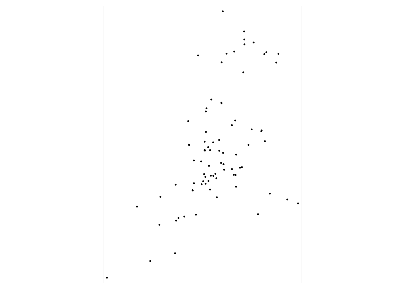

Make an interactive map of pharmacies

tmap_mode("view")

## tmap mode set to interactive viewing

qtm(pharm_fd_combined, "type_original")

Make a static map of the census tracts. First, remind ourselves the names of the variables.

names(tract_fulton_dekalb)

##  [1] "geo_id"            "name_tract_county" "pop"              
##  [4] "h_val_med_E"       "hh_inc_med_E"      "county_fips"      
##  [7] "area_4326"         "area_m2"           "atlanta_metro"    
## [10] "area_2240"         "area_ft2"          "area_mi2"         
## [13] "pop_dens_per_mi2"  "geometry"

tmap_mode("plot") #run again just in case it was changed above.

## tmap mode set to plotting

qtm(tract_fulton_dekalb)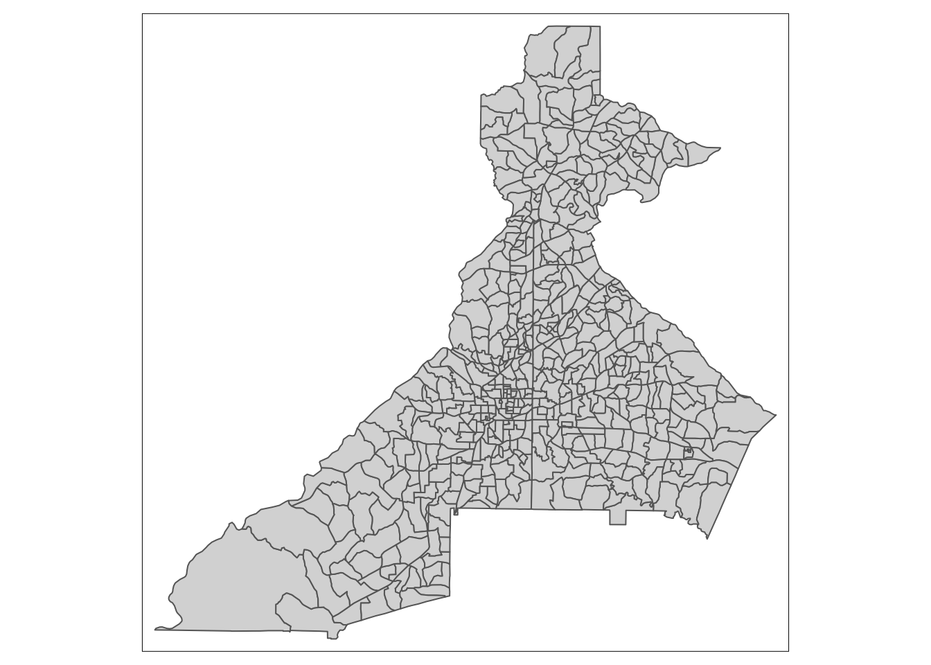

Make an interactive map of the census tracts.

tmap_mode("view") #run again just in case it was changed above.

## tmap mode set to interactive viewing

qtm(tract_fulton_dekalb)

1.2.1 Customize `qtm()`

All of the options for customization can be found here: https://rdrr.io/cran/tmap/man/qtm.html

Customize qtm for points. Change the shape of the point based on whether the point was originally imported as a polygon or a point by OpenStreetMap.

names(tract_fulton_dekalb)

##  [1] "geo_id"            "name_tract_county" "pop"              
##  [4] "h_val_med_E"       "hh_inc_med_E"      "county_fips"      
##  [7] "area_4326"         "area_m2"           "atlanta_metro"    
## [10] "area_2240"         "area_ft2"          "area_mi2"         
## [13] "pop_dens_per_mi2"  "geometry"

tmap_mode("plot")

## tmap mode set to plotting

qtm(pharm_fd_combined, symbols.shape = "type_original")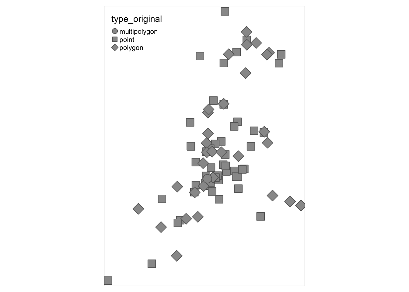

tmap_mode("view")

## tmap mode set to interactive viewing

qtm(pharm_fd_combined, symbols.shape = "type_original")

## Symbol shapes other than circles or icons are not supported in view mode.

Customize qtm for polygons (static)

tmap_mode("plot") #run again just in case it was changed above.

## tmap mode set to plotting

qtm(tract_fulton_dekalb, "h_val_med_E")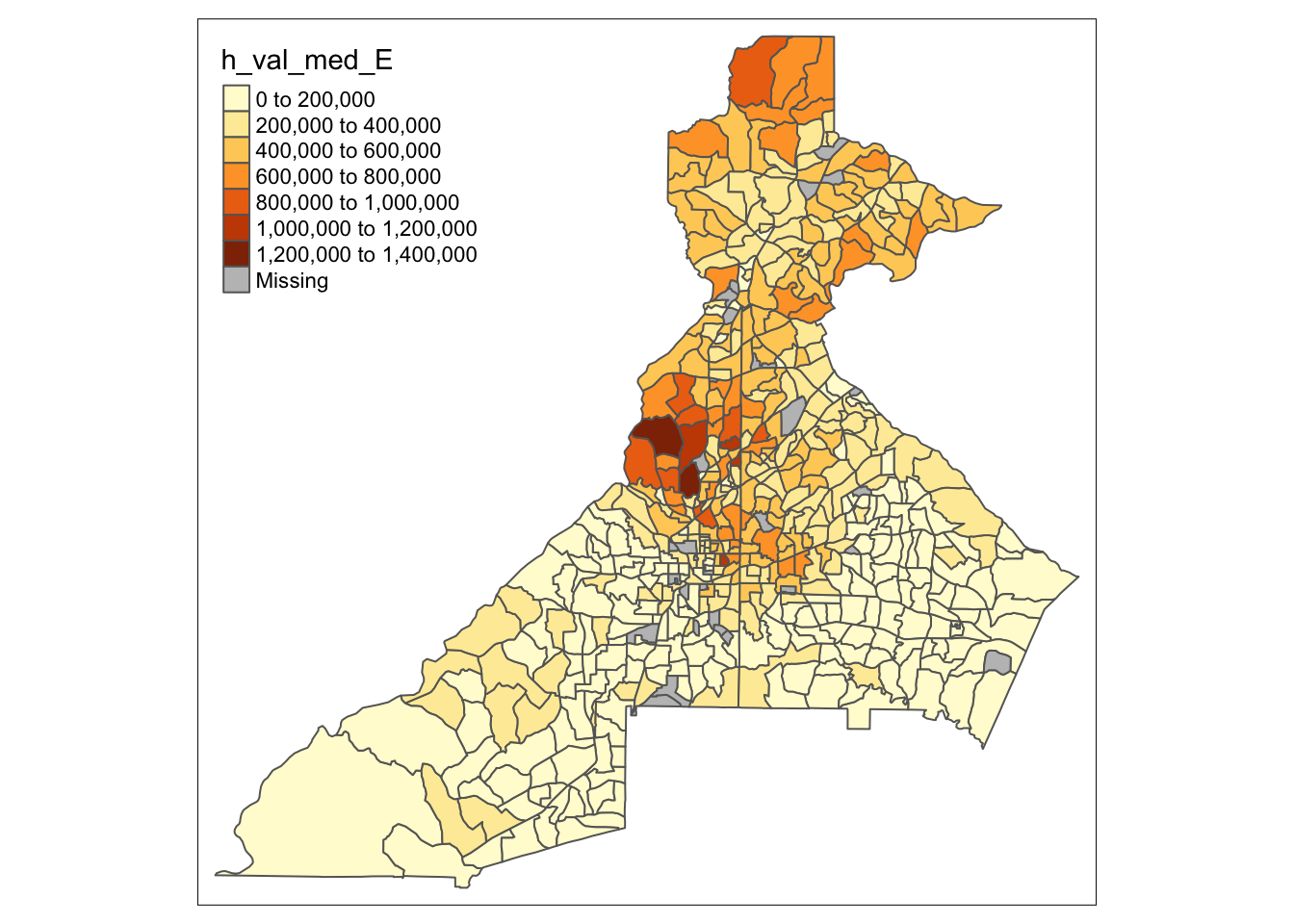

Customize qtm for polygons (interactive)

tmap_mode("view") #run again just in case it was changed above.

## tmap mode set to interactive viewing

qtm(tract_fulton_dekalb, "h_val_med_E")

1.3 More customization using `tmap()`

1.3.1 Adding multiple objects using `tmap()`

Static plot

tmap_mode("plot")

## tmap mode set to plotting

tm_shape(tract_fulton_dekalb)+
  tm_fill("h_val_med_E")+
  tm_borders()+
  
tm_shape(pharm_fd_combined)+
  tm_symbols(shape = "type_original")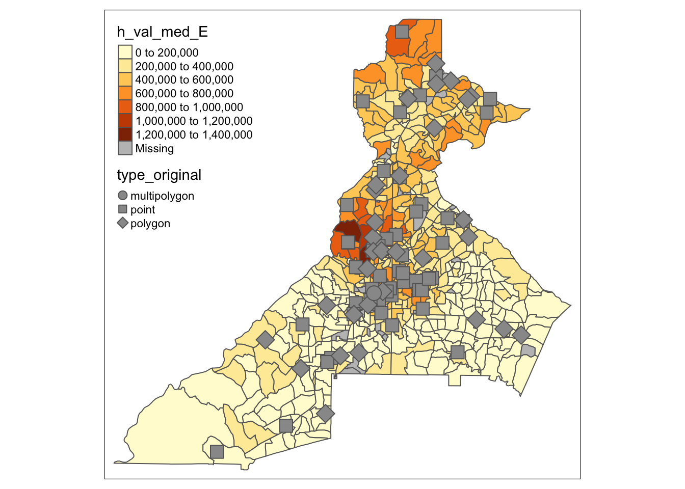

Interactive plot

tmap_mode("view")

## tmap mode set to interactive viewing

tm_shape(tract_fulton_dekalb) +
  tm_fill("h_val_med_E") +
  tm_borders()+
  
tm_shape(pharm_fd_combined)+
  tm_symbols(shape = "type_original")

## Symbol shapes other than circles or icons are not supported in view mode.

Comparison of R mapping methods: tmap vs mapview vs ggplot2

Michael D. Garber, PhD MPH

2022-08-23

1 tmap overview

1.1 Tmap mode

1.2 Quick maps using `qtm()`

1.2.1 Customize `qtm()`

1.3 More customization using `tmap()`

1.3.1 Adding multiple objects using `tmap()`

Comparison of R mapping methods: tmap vs mapview vs ggplot2

Michael D. Garber, PhD MPH

2022-08-23

1 tmap overview

1.1 Tmap mode

1.2 Quick maps using qtm()

1.2.1 Customize qtm()

1.3 More customization using tmap()

1.3.1 Adding multiple objects using tmap()

1.2 Quick maps using `qtm()`

1.2.1 Customize `qtm()`

1.3 More customization using `tmap()`

1.3.1 Adding multiple objects using `tmap()`