R for data wrangling 2: more dplyr and some tidycensus, mapview, and ggplot

In the last tutorial (https://michaeldgarber.github.io/teach-r/dplyr-1-nyt-covid.html), we learned the basics of using dplyr to wrangle a state-level dataset on COVID-19 cases and deaths. In this tutorial, we will build on that work to calculate cumulative and daily incidence per population. To grab population data, we’ll load census data using tidycensus. We also introduce sf, which is the workhorse library for wrangling spatial data in R. We’ll join the census data with our COVID-19 dataset and do some interactive mapping with mapview and finish with some ggplot2 graphs. To that end, let’s make sure we have the following packages installed:

library(tidyverse)
library(tidycensus)
library(mapview) #for interactive mapping
library(sf) #simple features for working with spatial (vector) data
library(viridis) #used to change color palettes
library(scales) #Used to help with the ggplot date axis below.
library(here) #working-directory mgmt in case we need to load data locally

1 Re-generate the NYT COVID-19 dataset we were working with before.

This simply repeats the code that we used in the previous tutorial to give us the same dataset we were working with.

Load the state-level data from the NYTimes GitHub repository the same way we did before.

nyt_state_url = "https://raw.githubusercontent.com/nytimes/covid-19-data/master/us-states.csv"
nyt_state_data = nyt_state_url %>% 
  url() %>% 
  read_csv()

This code reproduces our previous data wrangling where we calculated the daily number of incident cases.

Let’s also add a couple more variables that we may use later on (year, month, and week) using the convenient lubridate package. We use the year(), month(), and week() functions. Note these functions only work on date columns. Is the column called date formatted as a date? Yes.

class(nyt_state_data$date)

## [1] "Date"

Lubridate doesn’t automatically load when the tidyverse is loaded, so let’s load it:

library(lubridate)

## 
## Attaching package: 'lubridate'

## The following objects are masked from 'package:base':
## 
##     date, intersect, setdiff, union

nyt_state_wrangle = nyt_state_data %>% 
  group_by(state) %>% 
  arrange(date) %>% 
  rename(
    cases_cumul = cases,
    deaths_cumul = deaths
  ) %>% 
  mutate(
    cases_cumul_day_before = lag(cases_cumul),
    cases_incident = cases_cumul - cases_cumul_day_before,
    
    deaths_cumul_day_before = lag(deaths_cumul),
    deaths_incident = deaths_cumul - deaths_cumul_day_before,
    
    year = lubridate::year(date),
    month =lubridate::month(date),
    week = lubridate::week(date) #week of the year (i.e, 1-52)
  ) %>% 
  ungroup() %>% 
  arrange(state, date)

Did year, month, and week get created as expected?

nyt_state_wrangle %>% 
  dplyr::select(date, year, month, week)

## # A tibble: 50,014 × 4
##    date        year month  week
##    <date>     <dbl> <dbl> <dbl>
##  1 2020-03-13  2020     3    11
##  2 2020-03-14  2020     3    11
##  3 2020-03-15  2020     3    11
##  4 2020-03-16  2020     3    11
##  5 2020-03-17  2020     3    11
##  6 2020-03-18  2020     3    12
##  7 2020-03-19  2020     3    12
##  8 2020-03-20  2020     3    12
##  9 2020-03-21  2020     3    12
## 10 2020-03-22  2020     3    12
## # … with 50,004 more rows
## # ℹ Use `print(n = ...)` to see more rows

2 Load state-level census data using tidycensus

Tidycensus is a convenient package that allows census data to be downloaded into R at various geographic scales (e.g., state, county, census tract). The online material by the package author has great examples: https://walker-data.com/tidycensus/.

Use of tidycensus requires a key to access the U.S. Census API, which can be obtained for free here: https://api.census.gov/data/key_signup.html.

You will get a confirmation email with your key asking you to activate it, and then hopefully you see something like this:

The first time you use the key on your computer, enter this line of code, entering the key you received by email:

tidycensuscensus_api_key("your_census_key_here", install=TRUE)

Tidycensus lets the user specify

• the survey (American Community Survey or U.S. Census),
• the corresponding time period for that survey, the target geographic resolution and extent,
• the census variables to be downloaded, and
• whether or not the returned file will include the corresponding spatial data for the geographic units.

2.1 Brief introduction to sf

By specifying geometry=TRUE, an sf object will be returned representing the object for the chosen geography. If geometry=FALSE, then only the aspatial data will be returned. sf (or simple feature) objects have become the standard data structure for managing spatial data in R. We will cover sf objects more in a separate tutorial (https://michaeldgarber.github.io/teach-r/3-sf-atl-pharm.html). I would also encourage you to review these resources on sf:

• The main landing page maintained by the package author, Edzer Pebesma: https://r-spatial.github.io/sf/

• This chapter by Lovelace, Nowosad, and Muenchow: https://geocompr.robinlovelace.net/spatial-class.html. In fact, I highly recommend their whole book: https://geocompr.robinlovelace.net/.

• Here is another book written by an economist that I have found to be a great resource. The link to the chapter on sf, specifically, is here: https://tmieno2.github.io/R-as-GIS-for-Economists/vector-basics.html

One great aspect of sf objects–as compared with the sp package, the previous standard–is that spatial data can be handled as you would any other rectangular dataframe. An sf object is like a data.frame or tibble with an added column representing the geometry for that observation. The data structure of sf makes it straightforward to integrate spatial data into a typical data-wrangling workflow, during which you might add new variables, filter on a variable, or merge with additional data.

2.2 Get state-level population data

Without further adieu, let’s run the tidycensus function get_acs() to return state-level population data (2015-2019 5-year estimates) from the American Community Survey:

#Run this to save the data locally for speed.
options(tigris_use_cache = TRUE) 

#One way I keep track of whether an object has geometry associated with it to add a _geo suffix to the name.
pop_by_state_geo =tidycensus::get_acs(
  year=2019,
  variables = "B01001_001", #total population
  geography = "state",
  geometry = TRUE #to grab geometry
)

A convenient way to search through the census variables is to use the load_variables function, as described here: https://walker-data.com/tidycensus/articles/basic-usage.html.

vars_acs_2019 = tidycensus::load_variables(2019, "acs5", cache = TRUE)
View(vars_acs_2019)

2.2.1 Load the data from a local folder in case tidycensus::get_acs() did not work.

Note: if tidycensus::get_acs() returned an error because the Census key did not work, tidycensus did not load, or for any other reason, please feel free to download a version of pop_by_state_geo from this Dropbox folder:

I would then suggest saving the file (pop_by_state_geo.RData) to a folder within your R Studio project’s directory. For example, I would save save it to a folder called ‘data-input’ one level beneath the folder containing the .Rproj file for this project and would then load the data like this, using here::here() to set the working directory:

setwd(here("data-input"))
load("pop_by_state_geo.RData")

Confirm the data are an sf object (simple feature) and explore the data.

class(pop_by_state_geo)

## [1] "sf"         "data.frame"

pop_by_state_geo

## Simple feature collection with 52 features and 5 fields
## Geometry type: MULTIPOLYGON
## Dimension:     XY
## Bounding box:  xmin: -179.1489 ymin: 17.88328 xmax: 179.7785 ymax: 71.36516
## Geodetic CRS:  NAD83
## First 10 features:
##    GEOID                 NAME   variable estimate moe
## 1     12              Florida B01001_001 20901636  NA
## 2     30              Montana B01001_001  1050649  NA
## 3     27            Minnesota B01001_001  5563378  NA
## 4     24             Maryland B01001_001  6018848  NA
## 5     45       South Carolina B01001_001  5020806  NA
## 6     23                Maine B01001_001  1335492  NA
## 7     15               Hawaii B01001_001  1422094  NA
## 8     11 District of Columbia B01001_001   692683  NA
## 9     44         Rhode Island B01001_001  1057231  NA
## 10    31             Nebraska B01001_001  1914571  NA
##                          geometry
## 1  MULTIPOLYGON (((-80.17628 2...
## 2  MULTIPOLYGON (((-116.0491 4...
## 3  MULTIPOLYGON (((-89.59206 4...
## 4  MULTIPOLYGON (((-76.05015 3...
## 5  MULTIPOLYGON (((-79.50795 3...
## 6  MULTIPOLYGON (((-67.32259 4...
## 7  MULTIPOLYGON (((-156.0608 1...
## 8  MULTIPOLYGON (((-77.11976 3...
## 9  MULTIPOLYGON (((-71.28802 4...
## 10 MULTIPOLYGON (((-104.0534 4...

2.3 A quick mapview

Another essential package in the sf workflow is mapview (https://r-spatial.github.io/mapview/index.html), which creates quick interactive maps. In just one line, we can interactively map the ACS state-level population data we just loaded.

The zcol argument colors the polygons (states, here) based on the value of the variable, estimate, which corresponds to the state’s population, as obtained from tidycensus. The default color palette for the visualization is viridis.

mapview(pop_by_state_geo, zcol = "estimate")

Note that mapview can also be used with the pipe, as we’ll see below.

pop_by_state_geo %>% #the object name and then the pipe
  mapview( #Note the "object" argument is implied by the pipe operator, so we don't need to type it within mapview after a pipe.
    zcol = "estimate" )#the column to be visualized

2.4 Wrangle the census data further to prep for the join with the NYT state-level COVID-19 data.

Let’s clean up the output from tidycensus to make it easier to link with the state-level COVID-19 data.

names(pop_by_state_geo)

## [1] "GEOID"    "NAME"     "variable" "estimate" "moe"      "geometry"

The variable corresponding to the state name is called NAME in the tidycensus output. Rename it to state so it can be more easily joined with the NYT data. Also note that there is a column with the variable name variable and another column for its estimate. It’s formatted this way because the default output from tidycensus is long-form data. That is, we could have downloaded several variables for each state, and each variable-state combination would receive its own row. We can consolidate these fields by dropping the variable column using dplyr::select() and renaming estimate to population. Finally, because GEOID may vary depending on the geographic unit, let’s explicitly remember it’s a two-digit FIPS code and call it fips_2digit.

names(nyt_state_wrangle)

##  [1] "date"                    "state"                  
##  [3] "fips"                    "cases_cumul"            
##  [5] "deaths_cumul"            "cases_cumul_day_before" 
##  [7] "cases_incident"          "deaths_cumul_day_before"
##  [9] "deaths_incident"         "year"                   
## [11] "month"                   "week"

Importantly, we can wrangle this sf object the same way we would a tibble. For example, here we use a pipe (%>%) and the dplyr verbs dplyr::rename(), dplyr::select(), and dplyr::mutate(). Within the select() function, we use the - sign to drop variables from our dataset.

pop_by_state_wrangle_geo = pop_by_state_geo %>%
  rename(
    fips_2digit = GEOID,
    state = NAME,
    population = estimate
  ) %>% 
  dplyr::select(-moe, -variable) %>% 
  #To simplify some of the maps below, create an indicator variable corresponding to the Continental 48.
  mutate(
    continental_48 = case_when(
      state %in% c("Alaska", "Hawaii", "Northern Mariana Islands", "Guam", "Virgin Islands", "Puerto Rico") ~ 0,
      TRUE ~ 1)    
    ) 

names(pop_by_state_wrangle_geo)

## [1] "fips_2digit"    "state"          "population"     "geometry"      
## [5] "continental_48"

2.5 Use mapview to visualize population.

To confirm the population data are as we expect, let’s map the state’s populations using mapview. The pipe operator, %>%, can also be used before a mapview() call. In this code, the sf object, pop_by_state_geo, and all subsequent changes we make it to it, e.g., after having used filter() here, are “piped” into the mapview() function. Another advantage of the pipe when using mapview is that you can visualize various subsets (or other variations) of your data without having to create a new object if you don’t intend to use that variation later.

The zcol argument specifies which variable to be visualized. As you may notice, mapview defaults to the viridis color palette.

pop_by_state_wrangle_geo %>%
  filter(continental_48==1) %>%   #Limit to continental 48 so the default zoom is more zoomed in.
  mapview( 
    zcol = "population" ) #Note the object argument is implied by the pipe operator.

3 Link the NYT COVID-19 data with the census data

Let’s link the NYTimes COVID-19 data with the census data two ways.

We will first map an overall summary of cumulative incidence per state population. To do that, we will re-run some of our summary estimates from the previous tutorial to calculate the total number of cumulative cases. We will then link the census population data to the NYTimes data by state using dplyr::left_join(). We will calculate a rate (cumulative cases per population) and visualize it using mapview.

3.1 Summarize NYT COVID-19 data by state and link with census data.

Recall, we went through several ways to calculate the cumulative number of cases by state in our previous code. Let’s group by state and take the max value using dplyr::summarise(). Using the pipe, we can do these steps without having to create intermediate datasets.

left_join() takes three arguments: the data frame (or tibble) on the left side (piped through here), the data frame it’s merging with on the right side (pop_by_state_wrangle_geo), and the key variable on which the two tibbles will be merged, which is state. Note left_join() can also join on a vector of (two or more) variables if your key is represented by a combination of variables: by = c("var1", "var2"). Here we need just one key variable.

We use sf::st_as_sf() to force the dataframe to be an sf object. We finally use mutate() to create new variables which calcualte the cumulative incidence of both cases and deaths per population.

nyt_by_state_w_pop_geo = nyt_state_wrangle %>% 
  group_by(state) %>% 
  summarise(
    cases_cumul = max(cases_cumul, na.rm=TRUE),
    deaths_cumul = max(deaths_cumul, na.rm=TRUE)
    ) %>% 
  #Recall, after we use group_by and summarise, the data go from a very big dataset 
  #with a row for each day-state combination to a smaller dataset with just a row for every state.
  left_join(pop_by_state_wrangle_geo, by = "state") %>% #This contains the geometry
  sf::st_as_sf() %>% 
  mutate(
    cases_cumul_per_pop = cases_cumul/population,
    deaths_cumul_per_pop = deaths_cumul/population
  )

3.1.1 Visualize cumulative incidence per population using mapview

Use mapview to visualize.

nyt_by_state_w_pop_geo %>%
  #Limit to continental 48 so the default zoom is more zoomed in.
  filter(continental_48==1) %>% 
  mapview(
    zcol = "cases_cumul_per_pop")

The variable cases_cumul_per_pop is visualized, and it looks like North Dakota has had a particularly high incidence rate. Note that this measure should not be interpreted as a proportion. The same person can be counted as a case multiple times and thus it would theoretically be possible for this measure to take values greater than 1. That is, this measure is no not the percentage of the population that has had Covid-19; that proportion would probably be lower. We have counts of cases, not person-level data, so we can’t determine what proportion of people have been a case.

This measure may be easier to interpret if we were to split the data into year increments, so we could then calculate incident cases per person-year.

3.1.2 Exercise 1: Calculate incident cases per person-year for each state.

Exercise: Calculate the number of incident cases per person-year for each state.

3.1.3 Tinker with mapview’s defaults.

Mapview’s main raison d’etre is as a quick workflow check, but it can also be used to make more refined maps. One can, for example, change the label of the visualized variable in the legend (layer.name=) or change the color palette (col.regions=). See options here: https://r-spatial.github.io/mapview/articles/articles/mapview_02-advanced.html. In the below map, I made those changes and flipped the direction of the viridis color palette using the direction argument so that dark purple is high incidence and yellow is low. Check out the viridis color palettes here: https://cran.r-project.org/web/packages/viridis/vignettes/intro-to-viridis.html. B corresponds to the inferno palette: https://rdrr.io/cran/scales/man/viridis_pal.html.

The output is not bad, and I have used mapview in public-facing documents. Some people prefer tmap, though, for publication-ready maps, as it more flexible. We will discuss tmap more in a subsequent session. (Also see this tmap demo by a colleague, Lance Owen: https://rpubs.com/lancerowen/ElegantCartography_1).

nyt_by_state_w_pop_geo %>%
  filter(continental_48==1) %>%   #Limit to continental 48 so the default zoom is more zoomed in.
  mapview(
    zcol = "cases_cumul_per_pop",
    layer.name = "Cumulative incidence per pop",
    #The palette function is from the viridis package.
    col.regions = viridis_pal(alpha = 1, begin = 0, end = 1, direction = -1, option = "B")
  )

3.1.4 Visualize using a ggplot2 histogram

In addition to this geographic visualization, we may also want a simple aspatial figure summarizing cumulative incidence per population using ggplot2. Guidance on ggplot is extensive throughout the internet, for example: http://www.cookbook-r.com/Graphs/, and https://ggplot2.tidyverse.org/. A detailed discussion of ggplot2 is outside of the current scope. Let’s make a quick histogram accepting the ggplot2 defaults to get a sense of the distribution of the cumulative incidence variable.

As with mapview, ggplot() can be used after a pipe, so, in the below code the object (nyt_by_state_w_pop_geo, after having been modified by the filter() function) is passed through to the ggplot() function. After we write the initial ggplot() function, additional layers are connected with a + . In this case, we are just visualizing one variable, cases_cumul_per_pop, which we specify using the aes() function. We then add a histogram layer using geom_histogram(). See here for more options to customize histograms.

In subsequent figures, we specify two variables in the aes(x=xvar, y=var) function and use different types of layers, e.g., geom_line(). Other types of layers include geom_point() for a scatterplot or geom_bar for a bar chart–and lots more.

nyt_by_state_w_pop_geo %>%
  filter(continental_48==1) %>%   #Limit to continental 48 so the default zoom is more zoomed in.
  ggplot(aes(x=cases_cumul_per_pop))+
  geom_histogram() 

## `stat_bin()` using `bins = 30`. Pick better value with `binwidth`.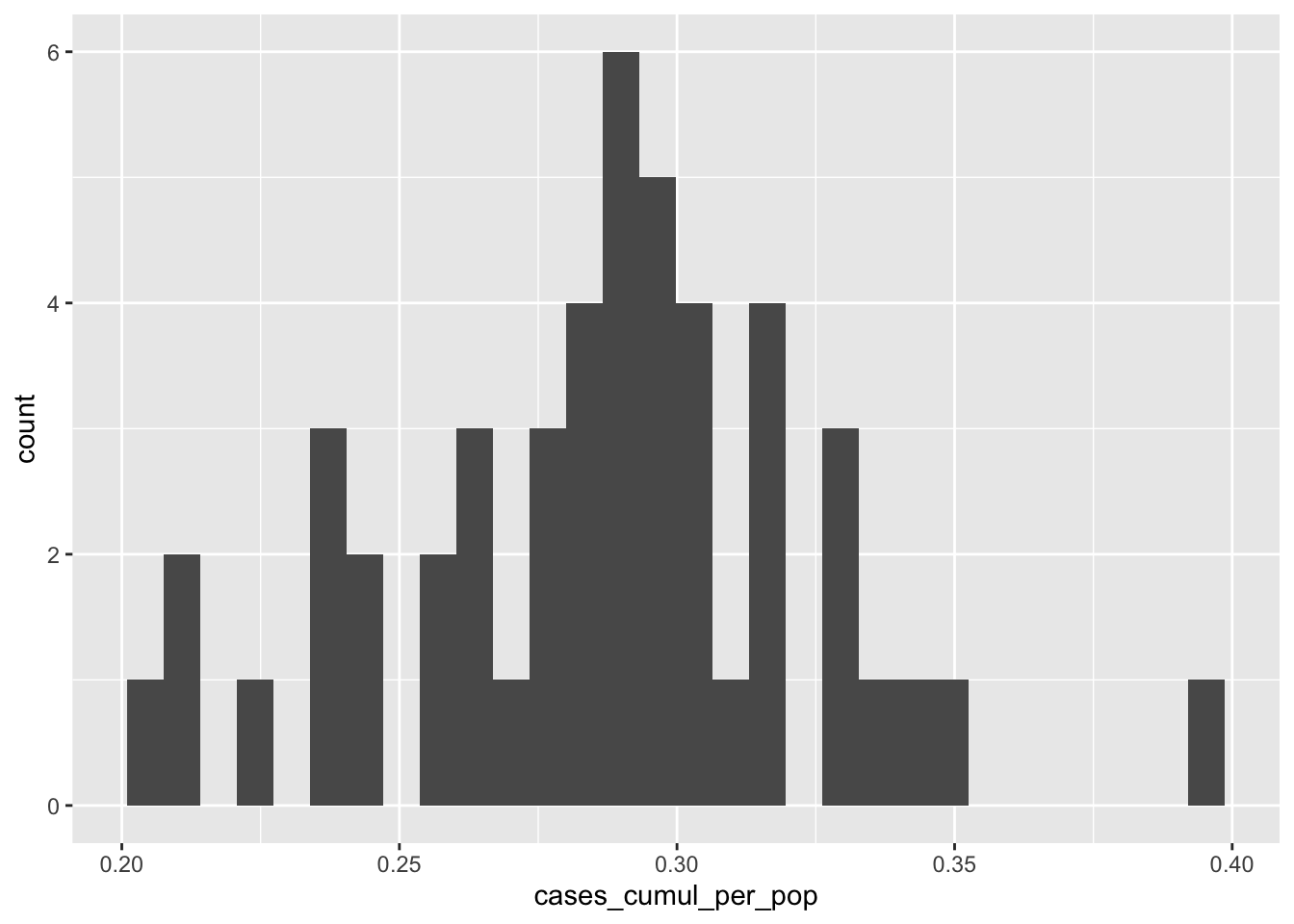

3.2 Link the daily NYT COVID-19 data with the population data to analyze temporal trends in incidence by state

In the above analysis, we collapsed over time. We might also be interested in time trends. In this section, we’ll keep the data in its daily format and link in the population data again.

Sometimes, there can be computer-processing benefits to dropping the geometry column, as it can make the file size quite a bit bigger. Since the daily data are thousands of observations, linking each day’s data with a corresponding geometry might be slow to work with. Let’s create a new state-population dataset without the geometry column before we link the population data to the daily COVID-19 data. Drop the geometry using the st_set_geometry(NULL) function from sf.

pop_by_state_wrangle_nogeo = pop_by_state_wrangle_geo %>% 
  sf::st_set_geometry(NULL)

Now, link the state-level population data to the daily COVID-19 data. Recall, the key variable for our dplyr::left_jon() is state. Calculate daily cumulative incidence of each outcome per population and the daily incidence rate of each outcome.

nyt_state_pop_wrangle = nyt_state_wrangle %>% 
  left_join(pop_by_state_wrangle_nogeo, by = "state") %>% 
  mutate(
    cases_cumul_per_pop = cases_cumul/population,
    deaths_cumul_per_pop = deaths_cumul/population,
    cases_incident_per_pop = cases_incident/population,
    deaths_incident_per_pop = deaths_incident/population 
  )

3.2.1 Visualize daily cumulative incidence per population for the continental 48 states using ggplot2.

Unlike the above histogram where we were only visualizing one variable, here, we’re visualizing cases_cumul_per_pop with respect to date, so in the ggplot() function, we write aes(x=date, y=cases_cumul_per_pop). Additional options are described in the comments below.

nyt_state_pop_wrangle %>% 
  filter(continental_48==1) %>%   
  ggplot( aes(x=date, y=cases_cumul_per_pop))+ #define the variables to be visualized.
  geom_line(aes(color = state)) + #color by state
  ylab("Cumulative COVID-19\n incidence\n per population") + #add a label to the y-axis
  xlab("Date")  + #add a label to the x-axis
  theme_bw() +  #convert to a black-and-white theme
  theme(legend.position="bottom") + #put the legend on the bottom of the chart.
  scale_x_date(date_breaks = "months" , date_labels = "%b-%y") + 
  theme(axis.text.x = element_text(angle = 90)) #rotate text on x-axis 90 degrees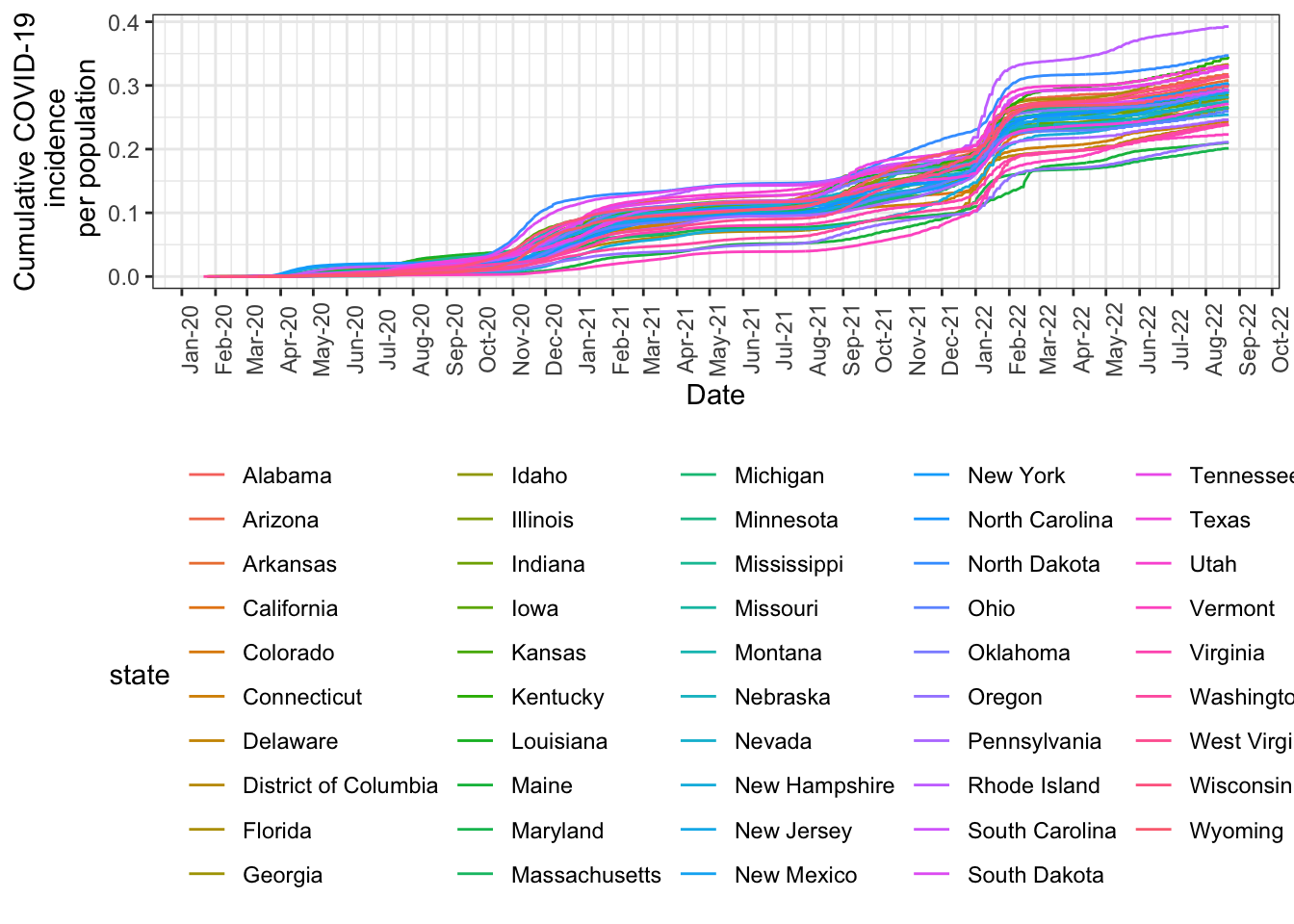

Recall incidence rate is the number of new cases per population per time period (day, here). We calculated it at the beginning of the code by subtracting the case count in a state on one day from the corresponding count from that state the day before.

nyt_state_pop_wrangle %>% 
  filter(continental_48==1) %>%   
  ggplot2::ggplot( aes(x=date, y=cases_incident_per_pop))+
  geom_line(aes(color = state)) +
  scale_x_date(date_breaks = "months" , date_labels = "%b-%y") +
  ylab("COVID-19\n incidence rate\n per population") +
  xlab("Date")  +
  theme_bw() +
  theme(legend.position="bottom") +
  theme(axis.text.x = element_text(angle = 90))

We could make those two charts prettier and easier to read, but graphing the two makes clear the distinction between the two measures (cumulative incidence vs incidence rate). Cumulative incidence only goes up, as expected, while incidence rate goes up and down.

One way to make the state-stratified data easier to read would be to break up the chart by group using a facet_wrap().

3.2.2 Exercise 2: Use facet_wrap to separate plots into groups.

Exercise: Divide the states into regions (e.g., using the classification here, and create line charts of cumulative incidence and incidence rate by state by region.

In April 2021, there was a reported spike in cases in Michigan. Let’s explore that by subsetting to the Great Lakes region, as we did previously. We can also subset to the year 2021 to further zoom into the relevant time period.

Note that, as we did above before our mapview() function, it is useful to pipe all of the data wrangling steps into the ggplot2() function instead of creating a new tibble, especially if you don’t think you’ll use that tibble for anything else. We do that below.

The spike in Michigan is indeed visible. This figure also illustrates how unstable and noisy daily values are.

nyt_state_pop_wrangle %>% 
  mutate(
    great_lakes = case_when(
      state == "Illinois" |
      state == "Indiana" |
      state == "Michigan" |
      state == "Minnesota" |
      state == "New York" |
      state == "Ohio" |
      state == "Pennsylvania" |
      state == "Wisconsin" ~ 1,
      TRUE ~ 0)) %>% 
  filter(great_lakes==1) %>% 
  filter(year == 2021) %>% 
  #Pipe the tibble into the ggplot function:
  ggplot( aes(x=date, y=cases_incident_per_pop))+
  geom_line(aes(color = state)) +
  ylab("COVID-19\n incidence rate\n per population") +
  xlab("Date")  +
  theme_bw() +
  scale_x_date(date_breaks = "months" , date_labels = "%b-%y") +
  theme(legend.position="bottom") +
  theme(axis.text.x = element_text(angle = 90))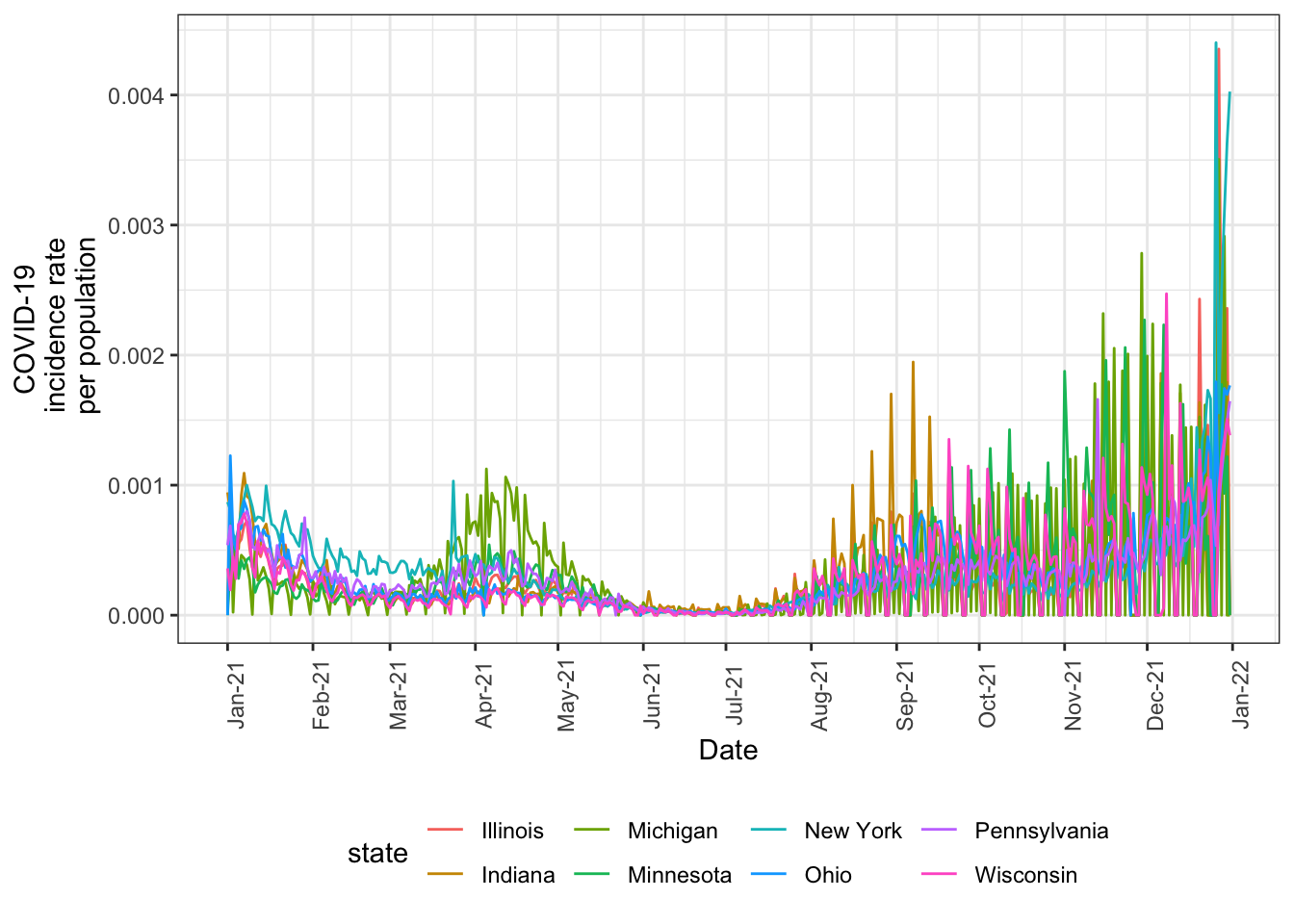

3.2.3 Exercise 3: Calculate and graph weekly incidence rate

Exercise: Weekly incidence rate is probably a more stable measure. How would we calculate that? Calculate weekly incidence rate and graph both overall (contiguous 48) and by state.

Copyright © 2022 Michael D. Garber