1 Outline

Introduction and pre-requisites
Install packages and download the data
Explore the NYT state COVID-19 data using dplyr

2 Introduction and pre-requisites

2.1 Purpose

The purpose of this tutorial is to learn the basics of dplyr in the context of an applied example with publicly available COVID-19 data from The New York Times.

2.2 Target audience

The target audience for this demo is someone with little to no experience using R. I will also assume no experience with any statistical programming language, although some experience with SAS or STATA would certainly not hurt. I imagine the target audience will have familiarity with the basics of data management in a spreadsheet-based program like Excel and may want to try using a programming-oriented tool for data management. For an excellent overview of why it can be preferable to analyze and manage data with a programming language rather than spreadsheet tools, please see the preliminary module of this series (https://michaeldgarber.github.io/teach-r/0-pre-reqs) or this great blog post by Jesse Adler.

2.3 What is dplyr?

Dplyr is a set of functions for managing and manipulating data in R. As stated on the webpage:

“dplyr is a grammar of data manipulation, providing a consistent set of verbs that help you solve the most common data manipulation challenges.”

There are several ways to manage data in R, including base R. I focus here on dplyr because it’s widely used and, I think, intuitive. Dplyr is part of the larger collection of packages called the tidyverse, which includes other popular packages like ggplot2. One advantage of dplyr is that, when combined with the pipe operator (explained below), it is quite human readable. Like good writing , it emphasizes the verbs (Zinsser, On Writing Well, Chapter 10).

2.4 The goal of this tutorial

The goal of this tutorial is to illustrate the basics of dplyr using publicly available data on COVID-19 incidence posted by The New York Times.

2.5 Prerequisites

R and RStudio are installed.

As a reminder:

To download R, go to CRAN and download R from the location nearest you: https://cran.r-project.org/mirrors.html.
Then, install RStudio Desktop (the free version) at this link: https://rstudio.com/products/rstudio/download .

You’re familiar with how to use the RStudio interface

Explore resources on dplyr. Finally, although we’ll cover the basics of dplyr here, you might peruse some of the excellent existing material on dplyr:

https://dplyr.tidyverse.org/ - The main webpage contains a short overview of the package and describes the key functions, aka verbs, as we will also do here.
https://dplyr.tidyverse.org/articles/dplyr.html - The vignette expands upon the main landing page with some examples.
https://r4ds.had.co.nz/transform.html - This book by Wickham and Grolemund is the authoritative guide to learning the tidyverse. The chapter on data transformation chapter covers dplyr, specifically.

3 Install packages and download the data

3.1 Install and load packages

Now that we have RStudio installed and up and running, our first step is to install packages, the basics of which we described in the previous module.

install.packages("tidyverse")

library(tidyverse)

## ── Attaching packages ─────────────────────────────────────── tidyverse 1.3.2 ──
## ✔ ggplot2 3.3.6     ✔ purrr   0.3.4
## ✔ tibble  3.1.8     ✔ dplyr   1.0.9
## ✔ tidyr   1.2.0     ✔ stringr 1.4.0
## ✔ readr   2.1.2     ✔ forcats 0.5.1
## ── Conflicts ────────────────────────────────────────── tidyverse_conflicts() ──
## ✖ dplyr::filter() masks stats::filter()
## ✖ dplyr::lag()    masks stats::lag()

3.2 Load the COVID-19 data from The New York Times

For this example, we will use COVID-19 data from The New York Times’ GitHub repository. There are a few datasets available at varying geographic scales. Let’s use their state-level dataset. The data include the number of cumulative cases and the number of cumulative deaths by state and day, beginning January 21, 2020.

We’ll load the data two ways, hoping at least one of them works.

3.2.1 Load the data directly from their Github repository

First, let’s try the fancy way, loading it directly from GitHub. Below, the first line of code defines an object, nyt_state_url to be the URL where the NYT data are located. The second line of code uses a base R function, url(), to parse that URL as a CSV. We then convert it from a CSV to an R object using read_csv(). read_csv() is a function in readr, another package in the tidyverse. Accordingly, the resulting output of these few lines of code will be a tibble, tidyverse speak for a “tidy table.” Basically, a tibble is a table, or data frame, with some opinionated formatting advantages that make it easy to work with.

Of note, the code below includes our first use of the %>% (read: pipe; keyboard shortcut: cmd+shift+m on Mac; ctrl+shift+m on PC) operator. The pipe operator is part of the magrittr package and is a key element of the tidyverse. The pipe separates the action-oriented functions, read_csv() and url() from the object, nyt_state_url. I think this separation makes the code easier to read, as I’ll discuss more in the next section.

Another side-note: I use the equals sign, =, when assigning new objects, because I think it’s easier to read type than R’s traditional assignment operator, <-. I’ve heard <- has advantages, but I’ve never had an issue using =.

nyt_state_url = "https://raw.githubusercontent.com/nytimes/covid-19-data/master/us-states.csv"

nyt_state_data = nyt_state_url %>% 
  base::url() %>% 
  readr::read_csv()

## Rows: 50014 Columns: 5
## ── Column specification ────────────────────────────────────────────────────────
## Delimiter: ","
## chr  (2): state, fips
## dbl  (2): cases, deaths
## date (1): date
## 
## ℹ Use `spec()` to retrieve the full column specification for this data.
## ℹ Specify the column types or set `show_col_types = FALSE` to quiet this message.

An alternative, equivalent, way to write that code is use the traditional nested parentheses. The nested parentheses aren’t so bad when just a few functions are used, but, as the number of functions increases, the nested parentheses become difficult to read.

nyt_state_url = "https://raw.githubusercontent.com/nytimes/covid-19-data/master/us-states.csv"
nyt_state_data = read_csv(url(nyt_state_url))

Either way we write it, we get a resulting dataset, nyt_state_data, which should be visible in the “Environment” pane (top right) of RStudio. It tells us that the data have 48,838 observations and 5 variables. (Again, I called this dataset on August 2, 2022; the number of observations will be higher in the future.)

As noted above, read_csv() is part of the readr package and returns a “tibble”. One benefit of using tibbles, as noted here, is that they can be printed without overwhelming the console. (This is not necessarily true of data frames more generally).

Let’s first confirm that nyt_state_data is a tibble using the base-R class() function, which returns the object’s class. The tibble object class is indicated by tbl_df. And then we can print the tibble by typing its name to get a sense of its dimensions (rows and columns) and what the variables look like.

At this writing, there are 48,838 observations and 5 columns. In the tibble print-out, the variable type (e.g., character, date, numeric) is listed in brackets just below the variable names.

We can also use the class() function from base R to return the type for a single column. The $ is a base-R function that extracts an element of an object by name.

class(nyt_state_data) #what type of object is it?

## [1] "spec_tbl_df" "tbl_df"      "tbl"         "data.frame"

nyt_state_data #print the tibble

## # A tibble: 50,014 × 5
##    date       state      fips  cases deaths
##    <date>     <chr>      <chr> <dbl>  <dbl>
##  1 2020-01-21 Washington 53        1      0
##  2 2020-01-22 Washington 53        1      0
##  3 2020-01-23 Washington 53        1      0
##  4 2020-01-24 Illinois   17        1      0
##  5 2020-01-24 Washington 53        1      0
##  6 2020-01-25 California 06        1      0
##  7 2020-01-25 Illinois   17        1      0
##  8 2020-01-25 Washington 53        1      0
##  9 2020-01-26 Arizona    04        1      0
## 10 2020-01-26 California 06        2      0
## # … with 50,004 more rows
## # ℹ Use `print(n = ...)` to see more rows

class(nyt_state_data$state) #character

## [1] "character"

3.2.2 Download the data I saved and read into R using `read_csv()`

If the direct call to NYT GitHub didn’t work, here’s a back-up way that should work to read the data into R. On August 2, 2022, I downloaded the data as a CSV. The file is called nyt_state_data_downloaded.csv in this Dropbox folder.

If needed, download the CSV and save locally to your computer. I would suggest saving to a sub-folder of this project, e.g., called “data-input”.

Then, use read_csv() to import the csv into R. As discussed in the last module, we can use the here package for this. So, if the .csv is in a folder in this project directory called, “data-input”, then this code should work to read it in:

library(here)
setwd(here("data-input"))
nyt_state_data = readr::read_csv("nyt_state_data_downloaded.csv")

3.2.3 Further explore the data using View() before manipulation with dplyr verbs.

Aside from printing the tibble by simply typing its name (nyt_state_data) we can use View (note the capital V) to view the data in a new window and interact with it in a more hands-on way. View() can be slow as the number of observations rises, but 40,000-ish shouldn’t be too bad. View() allows you to sort the data by values in the columns. We can sort the data by state in the View() window to confirm that the data are, in fact, cumulative: cases and deaths only increase.

View(nyt_state_data)

Here are some useful base-R commands for describing the basic aspects of the data.

nrow(nyt_state_data) #How many rows?

## [1] 48838

ncol(nyt_state_data) #How many columns?

## [1] 5

dim(nyt_state_data) #Get the table's dimensions, i.e., number of rows and columns.

## [1] 48838     5

names(nyt_state_data) #Return the names of the variables.

## [1] "date"   "state"  "fips"   "cases"  "deaths"

str(nyt_state_data) #Returns information about each variable's type (i.e., character vs numeric)

## spec_tbl_df [48,838 × 5] (S3: spec_tbl_df/tbl_df/tbl/data.frame)
##  $ date  : Date[1:48838], format: "2020-01-21" "2020-01-22" ...
##  $ state : chr [1:48838] "Washington" "Washington" "Washington" "Illinois" ...
##  $ fips  : chr [1:48838] "53" "53" "53" "17" ...
##  $ cases : num [1:48838] 1 1 1 1 1 1 1 1 1 2 ...
##  $ deaths: num [1:48838] 0 0 0 0 0 0 0 0 0 0 ...
##  - attr(*, "spec")=
##   .. cols(
##   ..   date = col_date(format = ""),
##   ..   state = col_character(),
##   ..   fips = col_character(),
##   ..   cases = col_double(),
##   ..   deaths = col_double()
##   .. )
##  - attr(*, "problems")=<externalptr>

4 Explore the NYT COVID-19 data using dplyr

In this section, I’ll introduce common dplyr verbs. We’ll first go through each verb one by one. Then, we’ll put them together in a sequence.

4.1 Essential dplyr verbs

The seven dplyr verbs I use the most are mutate(), filter(), select(), arrange(), group_by(), summarise(), and left_join():

mutate() adds new variables (or columns) that can be functions of existing variables.
filter() is essentially a subset operator. It picks rows based on their values.
select() selects variables (or columns) based on their names. It can also be thought of as a subset operator by column rather than by row.
arrange() sorts data. It orders the rows of a data frame by the values of selected columns. The default behavior is to sort ascending, meaning the lowest value will be on top. Use desc() within the arrange() function to sort descending. Importantly, arrange() will sort by group if data are grouped (below).
group_by() groups the table by a variable. group_by() is often but not always used with summarise(). When the two are used together, the result is akin to a pivot table in Excel.
summarise(), when used after group_by(), collapses the data, with rows corresponding to combinations of the grouping variables. And a new variable can be created within the summarise() function akin to a mutate(). Note that summarise() can also be used if data are not grouped. It can be used to compute a column-wise summary (e.g., mean, median, max) but will keep the dataset in its original form (i.e., not collapsed).
left_join() joins two tables together. It’s like a vlookup in Excel or, as the name implies, a JOIN in SQL. It’s distinct from the other verbs in this list in that it is a two-table verb. There are other types of joins, but I almost always use left_join(). A left join, specifically, keeps all of the values of the first datset and only those of the second dataset which correspond to the rows containing with a key common to the first object. In the below set of examples, left_join isn’t used. It is used in subsequent tutorials.

There are several other verbs within dplyr, but many, perhaps most, data-wrangling tasks can be done with just these seven tools.

(For the record, filter(), arrange(), select(), mutate(), and summarise() are considered to be the five key dplyr functions. I’ve added group_by() and left_join() because I use them so often.)

4.2 mutate()

For a demo of mutate(), let’s create a new variable called cases_plus_1, which is simply the number of cases plus 1. The first argument inside the mutate() call is the object to be operated on. And the second argument creates the new variable as a function of the old variable and, in this example, the number 1.

nyt_state_data_2 = mutate(nyt_state_data, cases_plus_1 = cases+1)

Adding the number 1 to the cases variable works because cases is a numeric variable. If cases were a character variable, it would not work.

class(nyt_state_data$cases)

## [1] "numeric"

Now let’s try the same thing but written with the pipe (%>%) operator. As mentioned above, the pipe brings the object out of the parentheses to focus on the action-oriented part of the function, making it easier to read.

nyt_state_data_2_pipe = nyt_state_data %>% 
  mutate(cases_plus_1 = cases+1)

Check our work by printing each one. They should be the same. Note the new column, cases_plus_1, in the objects nyt_state_data_2 and nyt_state_data_2_pipe.

nyt_state_data_2

## # A tibble: 48,838 × 6
##    date       state      fips  cases deaths cases_plus_1
##    <date>     <chr>      <chr> <dbl>  <dbl>        <dbl>
##  1 2020-01-21 Washington 53        1      0            2
##  2 2020-01-22 Washington 53        1      0            2
##  3 2020-01-23 Washington 53        1      0            2
##  4 2020-01-24 Illinois   17        1      0            2
##  5 2020-01-24 Washington 53        1      0            2
##  6 2020-01-25 California 06        1      0            2
##  7 2020-01-25 Illinois   17        1      0            2
##  8 2020-01-25 Washington 53        1      0            2
##  9 2020-01-26 Arizona    04        1      0            2
## 10 2020-01-26 California 06        2      0            3
## # … with 48,828 more rows
## # ℹ Use `print(n = ...)` to see more rows

nyt_state_data_2_pipe

## # A tibble: 48,838 × 6
##    date       state      fips  cases deaths cases_plus_1
##    <date>     <chr>      <chr> <dbl>  <dbl>        <dbl>
##  1 2020-01-21 Washington 53        1      0            2
##  2 2020-01-22 Washington 53        1      0            2
##  3 2020-01-23 Washington 53        1      0            2
##  4 2020-01-24 Illinois   17        1      0            2
##  5 2020-01-24 Washington 53        1      0            2
##  6 2020-01-25 California 06        1      0            2
##  7 2020-01-25 Illinois   17        1      0            2
##  8 2020-01-25 Washington 53        1      0            2
##  9 2020-01-26 Arizona    04        1      0            2
## 10 2020-01-26 California 06        2      0            3
## # … with 48,828 more rows
## # ℹ Use `print(n = ...)` to see more rows

Note, also that two new variables can be created in the same mutate() call. Each new variable is separated by a comma. For those familiar with SAS, this begins to look like a SAS data step.

nyt_state_data_2vars  = nyt_state_data %>% 
  mutate(
    cases_plus_1 = cases+1,
    cases_plus_2 = cases+2
    )
nyt_state_data_2vars

## # A tibble: 48,838 × 7
##    date       state      fips  cases deaths cases_plus_1 cases_plus_2
##    <date>     <chr>      <chr> <dbl>  <dbl>        <dbl>        <dbl>
##  1 2020-01-21 Washington 53        1      0            2            3
##  2 2020-01-22 Washington 53        1      0            2            3
##  3 2020-01-23 Washington 53        1      0            2            3
##  4 2020-01-24 Illinois   17        1      0            2            3
##  5 2020-01-24 Washington 53        1      0            2            3
##  6 2020-01-25 California 06        1      0            2            3
##  7 2020-01-25 Illinois   17        1      0            2            3
##  8 2020-01-25 Washington 53        1      0            2            3
##  9 2020-01-26 Arizona    04        1      0            2            3
## 10 2020-01-26 California 06        2      0            3            4
## # … with 48,828 more rows
## # ℹ Use `print(n = ...)` to see more rows

4.3 filter()

What if we only care about one state? Use filter() to subset values to Michigan. Again, we’ll do this with and without the pipe operator.

nyt_state_data_mi = filter(nyt_state_data, state == "Michigan")

nyt_state_data_mi_pipe = nyt_state_data %>% 
  filter(state == "Michigan")

A double equals sign, ==, is like asking the question is this equal to?. filter() evaluates where the statement, state == "Michigan", is true and returns rows with those values.

The number of observations decreased, as we’d expect. There are now 875 observations (at this writing).

nrow(nyt_state_data_mi)

## [1] 875

nrow(nyt_state_data_mi_pipe)

## [1] 875

4.4 select()

Let’s use select() to grab only the date variable. The syntax is to simply state the columns we want.

Side-note: select() is used by some other packages. To tell R that we want to use the select() function from dplyr, specifically, we use the :: operator and write dplyr::select(). We can use this syntax for any dplyr verb, e.g. dplyr::mutate() or dplyr::filter(), but select() is the only one where I frequently encounter conflicts with another package, so I usually leave it off the other ones for brevity.

Note that technically, the package_name::package_function() syntax can be used for packages that have not been attached via library() but otherwise are loaded via namespace.

The non-piped version:

date = dplyr::select(nyt_state_data, date)

And the piped version:

date_pipe = nyt_state_data %>% 
  dplyr::select(date)

Confirm that there’s just one variable using dim(date_pipe) or ncol().

dim(date_pipe) #dimensions

## [1] 48838     1

ncol(date_pipe) #number of columns

## [1] 1

There are several helpers that make select() easy to work with. Maybe we want all variables except for the number of deaths:

nyt_state_data_nodeaths = nyt_state_data %>% 
  dplyr::select(everything(), -deaths)
names(nyt_state_data)

## [1] "date"   "state"  "fips"   "cases"  "deaths"

names(nyt_state_data_nodeaths)

## [1] "date"  "state" "fips"  "cases"

4.5 arrange()

Arrange does not change values of the dataset. It just sorts the data. As a reminder, the NYT data include cumulative cases and cumulative deaths on that day in that state. We might also be interested in incident (i.e., new) cases or deaths by state. Let’s use arrange to help calculate daily cases and deaths using the lag() function.

In this code chunk, we’ll combine a few operations sequentially using the pipe, foregoing the nested parentheses approach. When many data-manipulation tasks are chained together, the value of the pipe becomes especially evident. From now on, I’ll adopt the teach-the-tidyverse-first philosophy and stick to its conventions, including the pipe.

4.6 group_by()

This code also uses group_by(), which does not sort the data, but it tells R to do any subsequent calculations “by group.”

Bonus question:

For this calculation, why is it better to group_by(state) and then arrange by date (i.e.: group_by(state) %>% arrange(date)) before the mutate() rather than an alternative method which could be to forego the grouping and simply arrange by state and then by state (arrange(state, date))? Try testing both ways and see what the value of the cases_cumul_day_before variable is on the first day of the data for a particular state.
It’s missing (correctly) when we first group_by(). In contrast, when we use arrange(state, date) without grouping, on the first day of data for a given state, cases_cumul_day_before takes the last day of data for its neighboring state in the alphabet. The lag() function doesn’t know that it shouldn’t take values from a different state. When we use group_by, the subsequent mutate() operates on each state as its own silo, which is what we want in this calculation.

Note, I’m creating a new dataset called nyt_state_wrangle. I tend to add a _wrangle to the name of datasets I’ve made significant changes to. (Tangent: Wikipedia page on origins of the term data wrangling).

nyt_state_wrangle = nyt_state_data %>% 

  #To calculate incident deaths, we will subtract the number of cumulative deaths on one day from the day before.
  #So let's group the data by state and then sort by date. Note it will default sort to ascending, meaning the earliest days will be on top.
  group_by(state) %>% 
  arrange(date) %>% 
  #Then calculate the number of incident deaths and incident cases on that day by subtracting the corresponding value from the day before.
  #Calculate the value from the day before using the lag() function, which grabs the value of one row up the data.
  #(We could have equivalently sorted descending and then used the lead() function.)
  #To explicitly differentiate between cumulative and incident deaths, let's rename the cases and deaths variables first using dplyr::rename()
  rename(
    cases_cumul = cases,
    deaths_cumul = deaths
  ) %>% 
  mutate(
    cases_cumul_day_before = lag(cases_cumul),
    cases_incident = cases_cumul - cases_cumul_day_before,
    
    deaths_cumul_day_before = lag(deaths_cumul),
    deaths_incident = deaths_cumul - deaths_cumul_day_before
  ) %>% 
  ungroup() %>% 
  #For visual convenience, now sort the data by state by date
  arrange(state, date)

nyt_state_wrangle

## # A tibble: 48,838 × 9
##    date       state   fips  cases_cumul deaths…¹ cases…² cases…³ death…⁴ death…⁵
##    <date>     <chr>   <chr>       <dbl>    <dbl>   <dbl>   <dbl>   <dbl>   <dbl>
##  1 2020-03-13 Alabama 01              6        0      NA      NA      NA      NA
##  2 2020-03-14 Alabama 01             12        0       6       6       0       0
##  3 2020-03-15 Alabama 01             23        0      12      11       0       0
##  4 2020-03-16 Alabama 01             29        0      23       6       0       0
##  5 2020-03-17 Alabama 01             39        0      29      10       0       0
##  6 2020-03-18 Alabama 01             51        0      39      12       0       0
##  7 2020-03-19 Alabama 01             78        0      51      27       0       0
##  8 2020-03-20 Alabama 01            106        0      78      28       0       0
##  9 2020-03-21 Alabama 01            131        0     106      25       0       0
## 10 2020-03-22 Alabama 01            157        0     131      26       0       0
## # … with 48,828 more rows, and abbreviated variable names ¹deaths_cumul,
## #   ²cases_cumul_day_before, ³cases_incident, ⁴deaths_cumul_day_before,
## #   ⁵deaths_incident
## # ℹ Use `print(n = ...)` to see more rows

4.6.1 group_by() (continued)

group_by() is often but not always used in combination with summarise(). We can use group_by() without summarise() to extract the total number of cases and deaths for each state. The last day of data for each state contains the cumulative total. After having sorted the data descending by date using dplyr::arrange(desc(date)), we use dplyr::group_by(state) to group the data by state and then dplyr::slice() to take the first row of data by group. In the next code chunk, we calculate the same cumulative total using the incident totals calculated above.

To incorporate our changes to the data modified above, first set the new dataset (nyt_last_day_by_state) equal to nyt_state_wrangle.

nyt_last_day_by_state = nyt_state_wrangle %>% 
  arrange(desc(date)) %>% #Use desc() to sort it by date descending, meaning the most recent day will be on the top of the dataset.
  group_by(state) %>% 
  slice(1) #The number 1 grabs the top row

nyt_last_day_by_state

## # A tibble: 56 × 9
## # Groups:   state [56]
##    date       state        fips  cases…¹ death…² cases…³ cases…⁴ death…⁵ death…⁶
##    <date>     <chr>        <chr>   <dbl>   <dbl>   <dbl>   <dbl>   <dbl>   <dbl>
##  1 2022-08-01 Alabama      01     1.42e6   19891  1.42e6       0   19891       0
##  2 2022-08-01 Alaska       02     2.87e5    1270  2.87e5       0    1270       0
##  3 2022-08-01 American Sa… 60     7.47e3      33  7.47e3       0      33       0
##  4 2022-08-01 Arizona      04     2.20e6   30768  2.20e6       0   30768       0
##  5 2022-08-01 Arkansas     05     9.05e5   11719  9.04e5     582   11719       0
##  6 2022-08-01 California   06     1.07e7   93651  1.07e7   13280   93613      38
##  7 2022-08-01 Colorado     08     1.61e6   13198  1.60e6    2233   13194       4
##  8 2022-08-01 Connecticut  09     8.55e5   11102  8.55e5     352   11102       0
##  9 2022-08-01 Delaware     10     2.95e5    3024  2.94e5     867    3024       0
## 10 2022-08-01 District of… 11     1.63e5    1364  1.63e5     173    1364       0
## # … with 46 more rows, and abbreviated variable names ¹cases_cumul,
## #   ²deaths_cumul, ³cases_cumul_day_before, ⁴cases_incident,
## #   ⁵deaths_cumul_day_before, ⁶deaths_incident
## # ℹ Use `print(n = ...)` to see more rows

#How many rows does the data have? The data should contain one row for each state or territory, since we grouped by state.
nrow(nyt_last_day_by_state)

## [1] 56

To see the difference between using and not using group_by(), try this code chunk. It will just grab the top row of the whole dataset, not the top row of each group.

nyt_last_day  = nyt_state_wrangle %>% 
  arrange(desc(date)) %>% 
#  group_by(state) %>% #This comments out the code so this part doesn't run.
  slice(1) #The number 1 grabs the top row

nrow(nyt_last_day)

4.6.2 group_by() and summarise()

Now, let’s use group_by() and summarise() together. The syntax of summarise() is similar to mutate() in that it creates a new variable with each equals sign. As with mutate(), several new variables can be created in a single summarise(), with each equality separated by a comma.

Let’s calculate three grouped summaries:

the average number of incident cases per day by state,
the cumulative number of cases by state (way 1) by summing incident cases,
the cumulative number of cases by state (way 2) by taking the maximum value of the number of cumulative cases.

Note that we have already found the cumulative number of cases above using arrange(), group_by(), and slice(). So here are two more options.

sum(), mean(), and max() are arithmetic functions in base R. In these functions, it’s good practice state na.rm=TRUE unless there’s a good reason not to. This argument stands for “remove missings equals true”. The default behavior of these arithmetic functions is to include missing values in the calculation (na.rm = FALSE), which means the arithmetic summary will also return a missing (e.g., 2+missing=missing), and that is typically not the desired outcome.

names(nyt_state_wrangle) #To remember the variable names.

## [1] "date"                    "state"                  
## [3] "fips"                    "cases_cumul"            
## [5] "deaths_cumul"            "cases_cumul_day_before" 
## [7] "cases_incident"          "deaths_cumul_day_before"
## [9] "deaths_incident"

nyt_cases_summary = nyt_state_wrangle %>% 
  group_by(state) %>% 
  summarise(
    cases_incident_average = mean(cases_incident, na.rm=TRUE),
    cases_cumul_way1 = sum(cases_incident, na.rm=TRUE),
    cases_cumul_way2 = max(cases_cumul, na.rm=TRUE)
    )

dim(nyt_cases_summary)

## [1] 56  4

nyt_cases_summary

## # A tibble: 56 × 4
##    state                cases_incident_average cases_cumul_way1 cases_cumul_way2
##    <chr>                                 <dbl>            <dbl>            <dbl>
##  1 Alabama                              1635.           1424405          1424411
##  2 Alaska                                329.            286792           286793
##  3 American Samoa                         23.9             7470             7471
##  4 Arizona                              2393.           2196428          2196429
##  5 Arkansas                             1036.            904512           904513
##  6 California                          11658.          10713332         10713333
##  7 Colorado                             1827.           1605856          1605858
##  8 Connecticut                           976.            854933           854934
##  9 Delaware                              338.            294907           294908
## 10 District of Columbia                  186.            162691           162692
## # … with 46 more rows
## # ℹ Use `print(n = ...)` to see more rows

The number of rows is equal to the number of groups. Washington D.C. and some territories are included, so the number of groups is above 50. The data used to include the column date, but we have collapsed over date here. When group_by() and summarise() are used together, the number of rows in the data will be equal to the number of groups.

The number of variables is four: the grouping variable (state) and each of the summary measures we calculated for each state.

Note that the two cumulative values differ slightly for some of the states. This discrepancy could be explained by the nuances of the NYT’s reporting system, which contains a mix of both probable and confirmed cases. The most trustworthy value is probably cases_cumul_way2, which takes the most recent reported cumulative value.

4.6.3 group_by() and summarise() (continued)

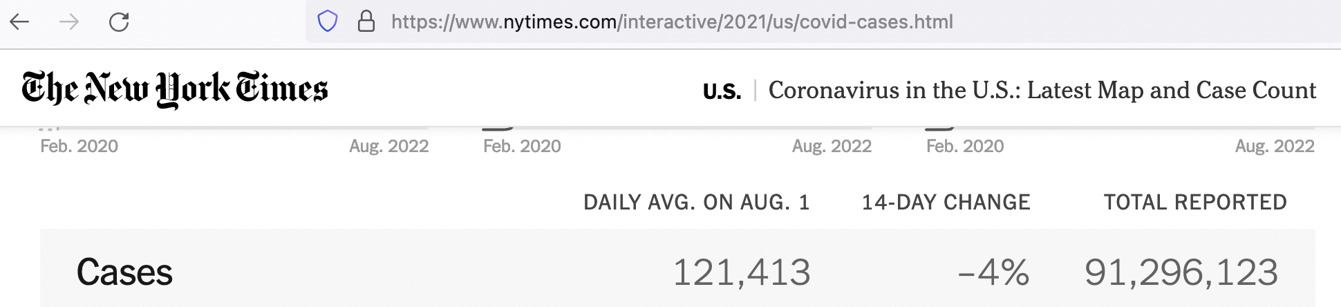
The group-by-summarise syntax can also be applied if we want to calculate overall summary estimates of the whole dataset. For example, as a double check, we can check to confirm the data we’re using lines up with what the NYT is reporting on their website for the total number of cumulative cases to date.

At this writing (8/2/22), NYT reports a total of ~91.3 million cases (https://www.nytimes.com/interactive/2021/us/covid-cases.html). Can we reproduce that? To summarize over the whole dataset, create a dummy variable with the same value for every observation and then sum over that variable.

nyt_cases_overall = nyt_state_wrangle %>% 
  group_by(state) %>% 
  summarise(cases_cumul = max(cases_cumul, na.rm=TRUE)) %>% 
  ungroup() %>% 
  mutate(dummy=1) %>%
  group_by(dummy) %>% 
  summarise(cases_cumul = sum(cases_cumul, na.rm=TRUE))
    

nyt_cases_overall

## # A tibble: 1 × 2
##   dummy cases_cumul
##   <dbl>       <dbl>
## 1     1    91296149

Confirmed. The total cumulative number of cases at this writing (8/2/22) is 91,296,149, which is about what they’re reporting on their website today (~91.3 million). Note this total includes the cases from Guam, Northern Mariana Islands, Puerto Rico, and the Virgin Islands.

4.7 All together now in an example using `case_when()`

Goal: calculate the total number of deaths in each state in the Great Lakes Region: Illinois, Indiana, Michigan, Minnesota, New York, Ohio, Pennsylvania, and Wisconsin. Do it all in one sequential pipe. In this code, I’ll introduce the case_when() function, which is a useful way to create new variables conditional on values of other variables.

Also note the use of the “or” operator, |.

Filtering the data to the subset of states in the Great Lakes Region could be done a few different ways. With complicated subsets, I prefer to create an indicator variable and then filter values based on that indicator variable, rather than putting all of the subset information into the filter() function.

So the code below uses mutate() to create a variable called great_lakes, which is equal to 1 if the state is in the Great Lakes region and 0 if not.

I also define this variable, great_lakes_alt, an alternative way, which is more concise but arguably less readable, using the %in% operator. That operator returns TRUE if an element belongs to a vector. A quick example to illustrate what %in% does:

x=c(1,2,3,4,5)
5%in%x

## [1] TRUE

6%in%x

## [1] FALSE

deaths_cumul_by_state_greatlakes = nyt_state_wrangle %>% 
  mutate(
    #If the condition is met, set the value to 1. If not -- confusingly expressed by TRUE -- set it to 0.
    great_lakes = case_when(
      state == "Illinois" |
      state == "Indiana" |
      state == "Michigan" |
      state == "Minnesota" |
      state == "New York" |
      state == "Ohio" |
      state == "Pennsylvania" |
      state == "Wisconsin" ~ 1,
      TRUE ~ 0),  #The parentheses closes this case_when function.
    #The comma outside the parentheses implies we have another variable to be created in the mutate function
    
    #Alternative way using the %in% operator: More but arguably less readable. The case_when function assigns a 1 wherever it's true.
    great_lakes_alt = case_when(
      state %in% c(
        "Illinois", "Indiana", "Michigan", 
        "Minnesota", "New York", "Ohio", 
        "Pennsylvania", "Wisconsin"
        ) ~ 1,
    TRUE ~0)
  ) %>% 
  
  filter(great_lakes==1) %>% 
  group_by(state) %>% 
  summarise(
    deaths_cumul = max(deaths_cumul, na.rm=TRUE)
  )

It should be a small dataset of 8 rows (one for each state) by 2 columns. Print to confirm:

deaths_cumul_by_state_greatlakes

## # A tibble: 8 × 2
##   state        deaths_cumul
##   <chr>               <dbl>
## 1 Illinois            38888
## 2 Indiana             24106
## 3 Michigan            37428
## 4 Minnesota           13293
## 5 New York            69628
## 6 Ohio                39035
## 7 Pennsylvania        46205
## 8 Wisconsin           14936

That concludes this tutorial. In our next tutorial (https://michaeldgarber.github.io/teach-r/2-dplyr-mapview-tidycensus.html), we’ll continue using dplyr and we’ll introduce tidycensus, mapview, and ggplot to use census data to visualize Covid-19 incidence per population.

R for data wrangling 1: learning the ground rules of dplyr with publicly available COVID-19 data

Michael D. Garber, PhD MPH

2022-08-23

1 Outline

2 Introduction and pre-requisites

2.1 Purpose

2.2 Target audience

2.3 What is dplyr?

2.4 The goal of this tutorial

2.5 Prerequisites

3 Install packages and download the data

3.1 Install and load packages

3.2 Load the COVID-19 data from The New York Times

3.2.1 Load the data directly from their Github repository

3.2.2 Download the data I saved and read into R using `read_csv()`

3.2.3 Further explore the data using View() before manipulation with dplyr verbs.

4 Explore the NYT COVID-19 data using dplyr

4.1 Essential dplyr verbs

4.2 mutate()

4.3 filter()

4.4 select()

4.5 arrange()

4.6 group_by()

4.6.1 group_by() (continued)

4.6.2 group_by() and summarise()

4.6.3 group_by() and summarise() (continued)

4.7 All together now in an example using `case_when()`

R for data wrangling 1: learning the ground rules of dplyr with publicly available COVID-19 data

Michael D. Garber, PhD MPH

2022-08-23

1 Outline

2 Introduction and pre-requisites

2.1 Purpose

2.2 Target audience

2.3 What is dplyr?

2.4 The goal of this tutorial

2.5 Prerequisites

3 Install packages and download the data

3.1 Install and load packages

3.2 Load the COVID-19 data from The New York Times

3.2.1 Load the data directly from their Github repository

3.2.2 Download the data I saved and read into R using read_csv()

3.2.3 Further explore the data using View() before manipulation with dplyr verbs.

4 Explore the NYT COVID-19 data using dplyr

4.1 Essential dplyr verbs

4.2 mutate()

4.3 filter()

4.4 select()

4.5 arrange()

4.6 group_by()

4.6.1 group_by() (continued)

4.6.2 group_by() and summarise()

4.6.3 group_by() and summarise() (continued)

4.7 All together now in an example using case_when()

3.2.2 Download the data I saved and read into R using `read_csv()`

4.7 All together now in an example using `case_when()`