Sampling counties for Streetlight analysis

1 Intro

1.1 Summary of approach

• Restrict sampling frame to counties of 48 contiguous United States above the 10th percentile of population (2,838) of the most rural group.
• Select all counties in the most urban stratum
• Sample the remaining counties stratified by the five remaining urban-rural categories and by the four regions (total of 4*5=20 strata). In each stratum, weight sampling proportional to the remaining population in that urban-rural-region stratum (prop_pop_elig_rem, in the code below).

An advantage of this approach is that, within each of the 20 strata, counties are randomly sampled, so in expectation, estimates will be representative of the full population of counties in that stratum. urban-rural-region stratum (n=20=4*5).

Load packages

library(tidyverse)
library(sf)
library(mapview)
library(RColorBrewer)
library(viridis)
library(tidycensus)
library(readxl)
library(here)
library(knitr)

1.2 Overview of dataset and variables

A dataset of counties with urban-rural codes (6 codes; 2013), regions (4 regions across US), divisions (9 across US) and SVI data. SVI data is from 2018, and urban rural codes are from 2013.

Urban-rural classification scheme is from here: https://www.cdc.gov/nchs/data_access/urban_rural.htm

1. Metropolitan counties: Large central metro counties in MSA of 1 million population that: 1) contain the entire population of the largest principal city of the MSA, or 2) are completely contained within the largest principal city of the MSA, or 3) contain at least 250,000 residents of any principal city in the MSA.
2. Large fringe metro counties in MSA of 1 million or more population that do not qualify as large central.
3. Medium metro counties in MSA of 250,000-999,999 population.
4. Small metro counties are counties in MSAs of less than 250,000 population.
5. Nonmetropolitan counties: Micropolitan counties in micropolitan statistical area.
6. Noncore counties not in micropolitan statistical areas.

9 divisions within 4 regions https://en.wikipedia.org/wiki/List_of_regions_of_the_United_States#Census_Bureau-designated_regions_and_divisions https://www2.census.gov/geo/pdfs/reference/GARM/Ch6GARM.pdf

2 Prep data

Make some new variables, remove a few variables, and exclude Alaska and Hawaii.

2.1 Load look-up tables from GitHub

To link in state abbreviations, urban-rural classification, and regions and divisions.

# Import these look-up tables from Github for convenience.
library(here)
source(here("scripts", "define-urls-look-up-tables.R"))

#Alternatively, they are available here:
us_state_fips_url = "https://raw.githubusercontent.com/michaeldgarber/lookups-county-state/main/us-state-fips.csv"
county_urban_rural_2013_url = "https://raw.githubusercontent.com/michaeldgarber/lookups-county-state/main/nchs-urban-rural-2013.csv"
region_division_url = "https://raw.githubusercontent.com/michaeldgarber/lookups-county-state/main/division-region.csv"

us_state_fips_lookup = us_state_fips_url %>% 
  url() %>% 
  read_csv()

county_urban_rural_2013_lookup = county_urban_rural_2013_url %>% 
  url() %>% 
  read_csv()

region_division_lookup = region_division_url %>% 
  url() %>% 
  read_csv()

names(us_state_fips_lookup)

## [1] "state_name"   "state_fips"   "state_abbrev"

names(county_urban_rural_2013_lookup)

## [1] "county_fips"           "cbsa_name"             "urban_rural_nchs_2013"

names(region_division_lookup)

## [1] "division_9_no"   "division_9_name" "region_4_no"     "region_4_name"  
## [5] "state_name"

2.2 Load county-level ACS data using tidycensus.

#Do not run this every time to avoid calling the census API frequently.
options(tigris_use_cache = TRUE) 
vars_acs_2019 <- load_variables(2019, "acs5", cache = TRUE)

county_geo =get_acs(
  year=2019,
  geography = "county",
  output = "wide", #make it wide form by default so variable names are in columns -   geography = "county",
  geometry = TRUE, #to grab geometry

  variables = c(
    
    pop  = "B01003_001", 
    
    #race
    race_pop_tot = "B02001_001", #denominator
    race_white = "B02001_002",
    race_black = "B02001_003",
    
    #median home value
    home_val_med = "B25077_001",
    home_val_med_tot = "B25075_001",
    
    #poverty
    poverty_pop_tot = "B17003_001", #the denominator for the poverty variable
    poverty_pop_below = "B17003_002",
    
    # means of transportation to work
    trans_to_work_pop_tot = "B08301_001",
    trans_to_work_car = "B08301_002",
    trans_to_work_public = "B08301_010",
    trans_to_work_bike = "B08301_018",
    trans_to_work_walk = "B08301_019",
    trans_to_work_other = "B08301_020"
  )
)

#save and re-load so don't have to call tidycensus every time
setwd(here("data-processed"))
save(county_geo, file = "county_geo.RData")

2.3 Set lower bound for population.

These bounds are determined later. Define them here (out of order) so that their values can be included in this data-prep step. Save the 10th and 20th population percentile of urban_rural_6=6. These are used as filters in future computations.

pop_ur_6_10th = 2815
pop_ur_6_20th = 4938    

2.4 Wrangle county-level data

setwd(here("data-processed"))
load("county_geo.RData") #saved above
county_wrangle_geo = county_geo %>% 
  #remove the margin-of-errors for this purpose
  dplyr::select(-ends_with("M")) %>% 
  rename(
    county_fips = GEOID, #The GEOID in this case is indeed a county FIPS code, as we imported counties.
    county_name = NAME,
         ) %>% 
  #for simplicity, remove the E suffix. E stands for estimate.
  rename_with(~str_remove(., 'E')) %>%  #https://stackoverflow.com/questions/45960269/removing-suffix-from-column-names-using-rename-all
  mutate(
    state_fips = str_sub(county_fips, 1,2), #obtain fips code for state
    
    #proportions for demographic variables and bike mode share
    prop_race_white = race_white/race_pop_tot,
    prop_race_black = race_black/race_pop_tot,
    prop_poverty = poverty_pop_below/poverty_pop_tot,
    prop_trans_to_work_walk = trans_to_work_walk/trans_to_work_pop_tot,
    prop_trans_to_work_bike = trans_to_work_bike/trans_to_work_pop_tot,
    
    #make into quantiles as well
    prop_trans_to_work_walk_cat = dplyr::ntile(prop_trans_to_work_walk, 4),
    prop_trans_to_work_bike_cat = dplyr::ntile(prop_trans_to_work_bike, 4),
    prop_race_white_cat = dplyr::ntile(prop_race_white, 4), 
    prop_poverty_cat = dplyr::ntile(prop_poverty, 4)
    
    ) %>% 
  #link in the state abbreviations, the nchs-urban-rural classifications, and the region-division lookup
  left_join(us_state_fips_lookup, by = "state_fips") %>% 
  left_join(county_urban_rural_2013_lookup, by = "county_fips") %>% 
  left_join(region_division_lookup, by = "state_name") %>% 
  rename(urban_rural_6 = urban_rural_nchs_2013) %>%   #simplify urban rural name. more descriptive on github.
  st_as_sf() %>% 
  st_transform(4326) %>% #make sure it's 4326 for area calculation
  mutate(
    continental_48 = case_when(
      state_name %in% c("Alaska", "Hawaii", "Northern Mariana Islands", "Guam", "Virgin Islands", "Puerto Rico") ~ 0,
      TRUE ~ 1),
    area_m2 = as.numeric(st_area(geometry)), #what is area in meters squared? 4326 is coordinate system, so meters are returned
    area_mi2 = area_m2/2589988.11, #square miles
    pop_per_mi2 = pop/area_mi2,
    pop_log = log(pop), #in case needed as a weight
    
    #indicator variables for above the 10th and 20th population percentile in the sixth urban-rural category
    pop_above_ur_6_10th = case_when(pop >= pop_ur_6_10th ~ 1, TRUE ~ 0 ),
    pop_above_ur_6_20th = case_when(pop >= pop_ur_6_20th ~ 1, TRUE ~ 0 ) ,
    
    #indicator variable for most urban classification or not
    ur_1 = case_when(
      urban_rural_6 ==1 ~1,
      TRUE ~0)
    
    ) %>% 
    #sort by population to note the top 150 and top 150
  arrange(desc(pop)) %>%
  mutate(
    pop_rank = row_number(),
    pop_top_150 = case_when(
           pop_rank <=150 ~ 1,
           TRUE ~ 0
         ),
    pop_top_200 = case_when(
           pop_rank <=200 ~ 1,
           TRUE ~ 0)
  )  %>% 
  #restrict to contiguous 48
  filter(continental_48==1)
  

#Make a version without geometry
county_wrangle_nogeo = county_wrangle_geo %>% 
  st_set_geometry(NULL) %>% 
  as_tibble()
county_geo_lookup = county_wrangle_geo %>% 
  dplyr::select(county_fips, geometry)

setwd(here("data-processed"))
save(county_wrangle_nogeo, file = "county_wrangle_nogeo.RData")
save(county_geo_lookup, file = "county_geo_lookup.RData")

2.5 Create sf objects for the regions and divisions

division_9_sf = county_wrangle_geo %>% 
  group_by(division_9_no) %>% 
  summarise(area_mi2 = sum(area_mi2, na.rm=TRUE)) %>% #like a dissolve
  st_cast()

region_4_sf = county_wrangle_geo %>% 
  group_by(region_4_no) %>% 
  summarise(area_mi2 = sum(area_mi2, na.rm=TRUE)) %>% 
  st_cast()

#Note these steps take some time. Save to avoid having to run the slow code
library(here)
setwd(here("data-processed"))
save(division_9_sf, file = "division_9_sf.RData")
save(region_4_sf, file = "region_4_sf.RData")

3 Check and explore data

3.1 Obtain lower bound of population as 10th percentile of most rural.

pop_dist_by_urban_rural_6 = county_wrangle_nogeo %>% 
  group_by(urban_rural_6) %>% 
  summarise(
    pop_min = min(pop, na.rm=TRUE),
    pop_10th = round(quantile(pop, probs = .1, na.rm=TRUE), digits = 0),
    pop_20th = round(quantile(pop, probs = .2, na.rm=TRUE), digits = 0),
    pop_25th = round(quantile(pop, probs = .25, na.rm=TRUE), digits = 0)
  )
options(digits =4)
library(knitr)
pop_dist_by_urban_rural_6 %>% 
  knitr::kable()

urban_rural_6	pop_min	pop_10th	pop_20th	pop_25th
1	157613	467485	663826	695333
2	4830	17295	28980	37572
3	1973	16372	26231	34105
4	728	10845	17045	20582
5	395	12825	22351	25072
6	98	2815	4938	6032

3.2 Explore the 9 divisions and 4 regions.

Map with ggplot rather than mapview for speed.

#Load strata maps
library(here)
setwd(here("data-processed"))
load(file = "division_9_sf.RData")
load(file = "region_4_sf.RData")

division_9_sf %>% 
  ggplot()+
  geom_sf(color = "black", fill = "azure4")+
  geom_sf_label(aes(label=division_9_no))+
  theme_bw()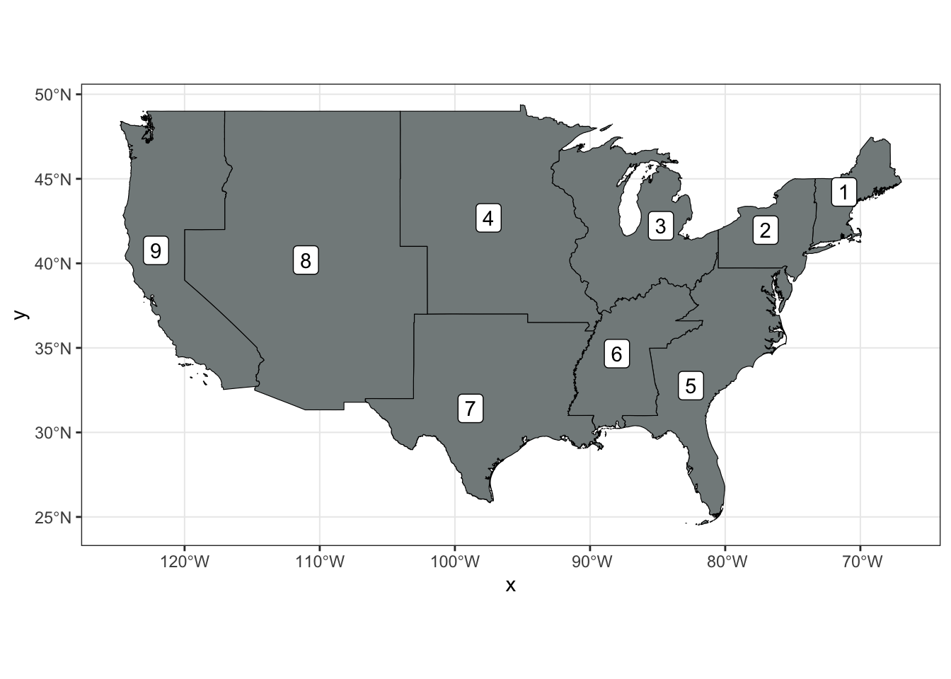

region_4_sf %>%
  ggplot()+
  geom_sf(color = "black", fill = "orange") +
  geom_sf_label(aes(label=region_4_no))+
  theme_bw()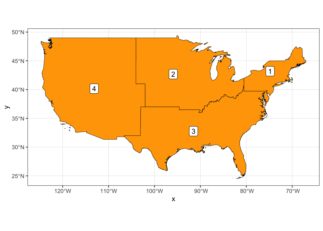

3.3 Number of counties and total population: contiguous 48

#marginal total to not be confused with the joint values below
n_counties_marg = county_wrangle_nogeo %>% 
  count() %>% 
  pull()
n_counties_marg

## [1] 3108

pop_marg_total = county_wrangle_nogeo %>% 
  mutate(dummy=1) %>%
  group_by(dummy) %>%
  summarise(pop_total = sum(pop, na.rm=TRUE)) %>%
  dplyr::select(-dummy) %>%
  ungroup() %>% 
  pull()
pop_marg_total

## [1] 322538633

3.4 Number of counties and total population: contiguous 48, excluding those in the bottom 10th percentile of the most rural classification?

#Total number of eligible counties to be sampled. Define as object for later use.
n_counties_marg_elig =county_wrangle_nogeo %>% 
  filter(pop_above_ur_6_10th==1) %>% 
  count() %>% 
  pull()

n_counties_marg_elig

## [1] 2959

pop_marg_elig = county_wrangle_nogeo %>% 
  filter(pop_above_ur_6_10th==1) %>% 
  mutate(dummy=1) %>%
  group_by(dummy) %>%
  summarise(pop = sum(pop, na.rm=TRUE)) %>%
  dplyr::select(-dummy) %>%
  ungroup() %>% 
  pull()

pop_marg_elig 

## [1] 322285160

3.5 Number of counties and population total by urban-rural classification

by_ur = county_wrangle_nogeo %>% 
  group_by(urban_rural_6) %>% 
  summarise(
    n_counties=n(),
    prop = n_counties/n_counties_marg_elig, #use overall here rather than restricting to the overall numbers.
    pop = sum(pop, na.rm=TRUE),
    prop_pop  =pop/ pop_marg_total) %>% 
  ungroup()

by_ur

n_counties_ur_1 = by_ur %>% 
  filter(urban_rural_6==1) %>% 
  dplyr::select(n_counties) %>% 
  pull()

The most urban category comprises 68 counties, which is 2% of the counties in the sampling frame and 31% of the population.

3.6 Histogram of population by urban-rural classification

It looks like every category has a long right tail. Most counties in each category are lower population. The most rural category especially has a right skew.

county_wrangle_geo %>% 
  ggplot(aes(pop))+
  geom_histogram() +
  facet_wrap(~urban_rural_6, scales = "free") + #allow axes to vary freely.
  scale_x_continuous(labels=scales::comma)+
  theme(axis.text.x = element_text(angle = 90))+
  ylab("Number of counties") +
  xlab("Population")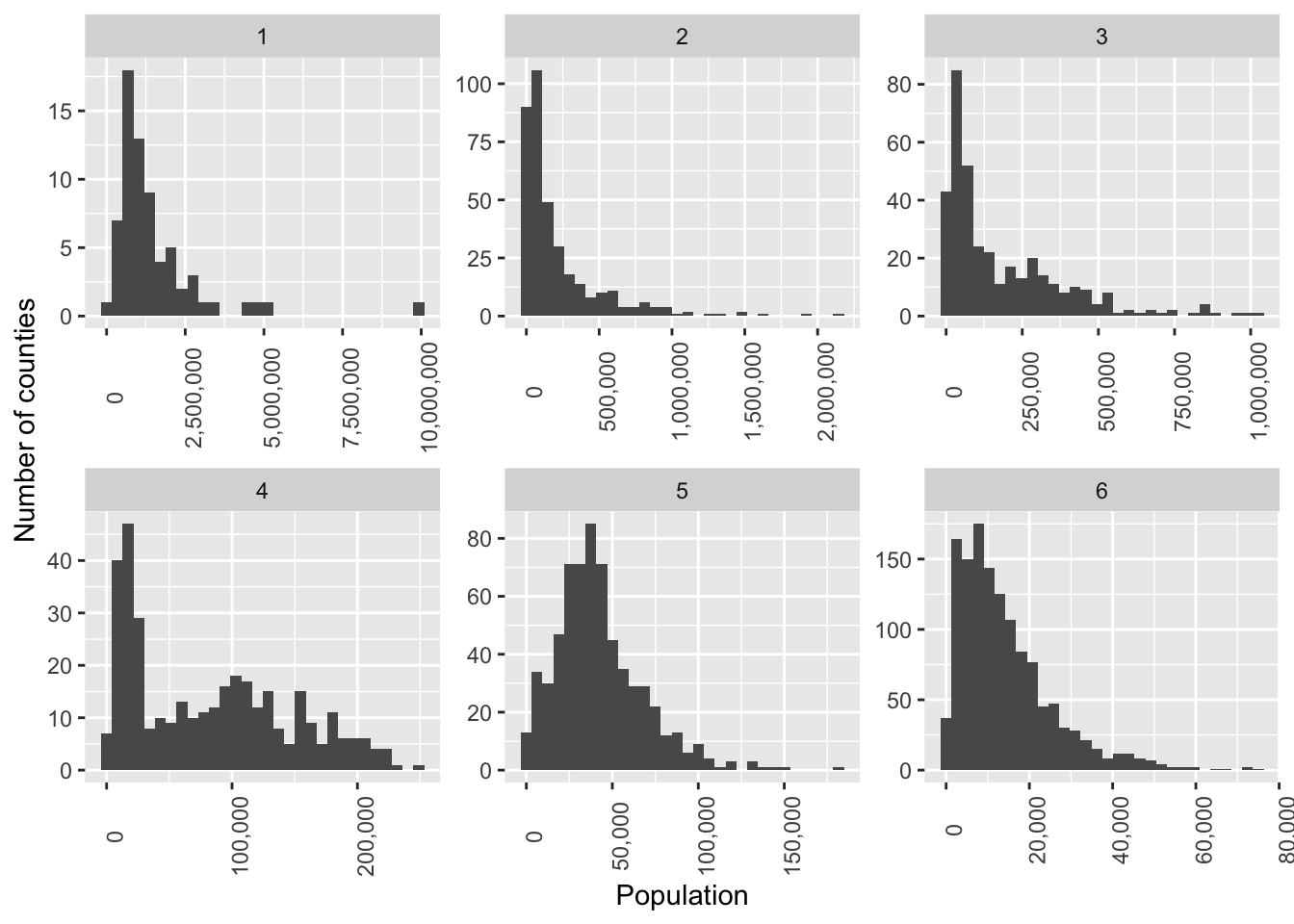

Examine logged version to see if has a more normal distribution. Could sample weighted by log(pop) if want to weight proportionally to population without such extreme weights.

county_wrangle_geo %>% 
  ggplot(aes(pop_log))+
  geom_histogram() +
  facet_wrap(~urban_rural_6, scales = "free") + #allow axes to vary freely.
  scale_x_continuous(labels=scales::comma)+
  theme(axis.text.x = element_text(angle = 90))+
  ylab("Number of counties") +
  xlab("Natural logarithm of population")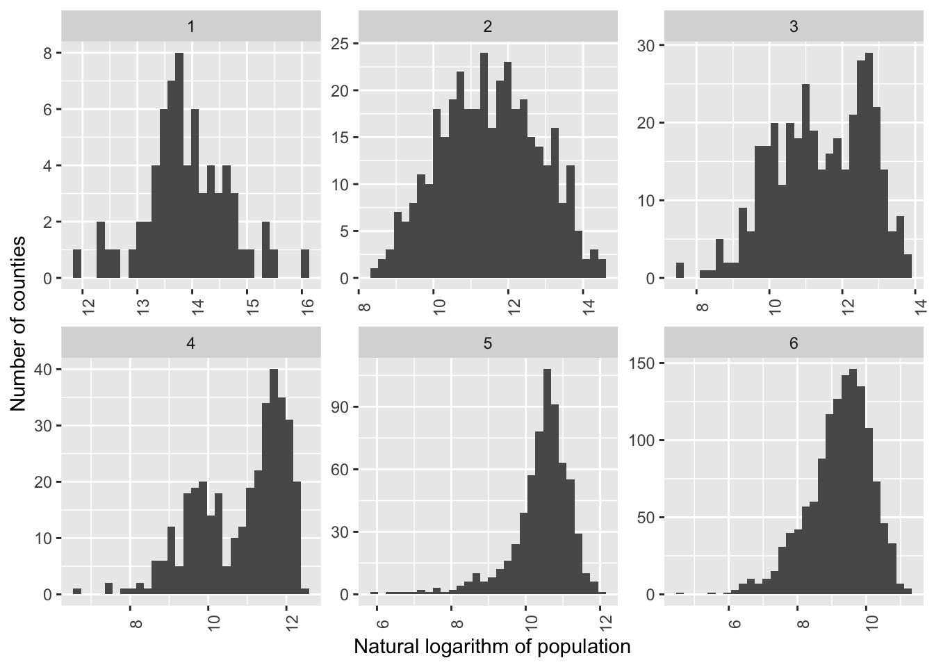

3.7 Map of population distribution among most urban counties

county_wrangle_geo %>% 
  filter(urban_rural_6==1) %>% 
  mutate(
    pop_urban_rural_cat = dplyr::ntile(pop, 4)
    )%>% 
  dplyr::select(state_abbrev, pop_urban_rural_cat) %>% 
  mapview(
    zcol = "pop_urban_rural_cat",
        layer.name = "Population quartiles (1=min-25th; 4=75th-max)",
        map.types = c("CartoDB.Positron"),
    lwd=1.5,
  col.regions = viridis_pal(alpha = 1, begin = .25, end = 1, direction = 1, option = "H"), #turbo :)
  popup = FALSE #for faster rendering
    )

4 Define sampling weights within urban-region-rural stratum after selecting the most urban stratum.

#Create some values for future use.
#The remaining eligible population and number of counties to be sampled after the most urban is selected.
margin_total_rem = county_wrangle_nogeo %>% #rem for remaining
  filter(pop_above_ur_6_10th==1) %>% 
  filter(ur_1==0) %>%
  group_by(ur_1) %>% 
  summarise(
    n_counties = n(),  
    pop = sum(pop, na.rm=TRUE))

pop_marg_elig_rem  = margin_total_rem %>% 
  dplyr::select(pop) %>% 
  pull()
n_counties_marg_elig_rem = margin_total_rem %>% 
  dplyr::select(n_counties) %>% 
  pull()
n_counties_left = 300- n_counties_ur_1 #the number of counties we have left.

urban_rural_region_strata = county_wrangle_nogeo %>% 
  filter(pop_above_ur_6_10th==1) %>% 
  filter(ur_1==0) %>%
  group_by(urban_rural_6, region_4_no) %>% 
  summarise(
    n_counties = n(), #remaining counties in the sampling frame by stratum
    pop_stratum = sum(pop, na.rm=TRUE)
  ) %>% 
  ungroup() %>% 
  mutate(
    #Note pop_marg_elig_rem is not in this dataset. It is a value created just above.
    #the proportion of the population remaining in each urban-rural-region stratum
    prop_pop_elig_rem =  pop_stratum/pop_marg_elig_rem, 
    n_counties_to_sample = n_counties_left*prop_pop_elig_rem,  #number of counties left times the proportion of remaining population in that stratum.
    n_counties_to_sample_rnd = round(n_counties_to_sample),  #for sample_n, we need a rounded version
    prop_counties_rem_to_sample = n_counties_to_sample/n_counties_marg_elig_rem,#the sampling fraction

    #re-calculate the proportion of counties actually sampling based on the rounded value
    #doing this because the rounded value is used in the sample_n function below. 
    #This variable can be used to calculate weights
    #for pooled estimates. Note it's not actually a rounded version of prop_counties_rem_to_sample. 
    #It's a re-calculated proportion based on the rounded value of n_counties_to_sample.
    prop_counties_rem_to_sample_rnd = n_counties_to_sample_rnd/n_counties_left,
    wt = 1/prop_counties_rem_to_sample_rnd, #weights (empirical). note that the most urban stratum would have a weight of 1.
    wt_prop = wt/sum(wt) #each weight's relative weight. sums to 1. easier than using the actual weight.
) 
options(scipen = 99, digits = 2) #set to fewer decimals before printing table


urban_rural_region_strata  

setwd(here("data-processed"))
save(urban_rural_region_strata, file = "urban_rural_region_strata.RData")


#Create a dataset of weights only.
wts = urban_rural_region_strata %>% 
  dplyr::select(urban_rural_6, region_4_no, wt, wt_prop)

Does the total number sampled in each stratum add up to the total remaining? No, due to rounding, 2 are missing.

n_counties_left

## [1] 232

urban_rural_region_strata %>%  
  mutate(dummy=1) %>%  
  group_by(dummy) %>%  
  summarise( n_counties_to_sample_rnd=sum(n_counties_to_sample_rnd)) %>% 
  pull(n_counties_to_sample_rnd)

## [1] 230

5 Draw sample

5.1 Draw one sample.

set.seed(123) #set seed so that the sample is the same each time.
samp = county_wrangle_nogeo %>% 
  filter(ur_1==0) %>% 
  filter(pop_above_ur_6_10th==1) %>% 
  left_join(urban_rural_region_strata, by = c("urban_rural_6", "region_4_no")) %>%
  group_by(urban_rural_6, region_4_no) %>% 
  #slice_sample is the more recent update, but sample_n is better for this application.
  #Use the solution by thc here: https://stackoverflow.com/questions/51671856/dplyr-sample-n-by-group-with-unique-size-argument-per-group/59186490#59186490l
  sample_n(
    size=n_counties_to_sample_rnd[1], 
    # the subset operator, [] takes the first value in that column by group. 
    replace=FALSE) %>%
  mutate(sampled=1)

nrow(samp)

## [1] 230

5.2 Map one instance of this sampling approach

mv_samp = samp %>% 
  left_join(county_geo_lookup, by = "county_fips") %>% 
  st_as_sf() %>% 
  dplyr::select(state_name, division_9_no, urban_rural_6, sampled) %>% 
  mapview(
    zcol = "urban_rural_6",
  layer.name = "Urban-rural classification",
          map.types = c("CartoDB.Positron")
  )

mv_ur_1 = county_wrangle_geo %>% 
  filter(ur_1==1) %>%
  mapview(
    layer.name = "urban-rural=1",
    col.regions="red")

mv_samp + mv_ur_1

6 Summarize results

6.1 Define a function to replicate the sampling.

draw_sample   <-function(s_id_val){
    sample_df = county_wrangle_nogeo %>% 
      filter(ur_1==0) %>% 
      filter(pop_above_ur_6_10th==1) %>% 
      left_join(urban_rural_region_strata, by = c("urban_rural_6", "region_4_no")) %>%
      group_by(urban_rural_6, region_4_no) %>% 
      #hmm, need to be able to vary sampling proportion by group - https://github.com/tidyverse/dplyr/issues/5299
      #slice_sample is the more recent dplyr update, but sample_n is better for this application.
      #Use the solution by thc here: https://stackoverflow.com/questions/51671856/dplyr-sample-n-by-group-with-unique-size-argument-per-group/59186490#59186490l
      sample_n(
  #the subset operator, [] takes the first value in that column by group. see above for definition.
        size=n_counties_to_sample_rnd[1], 
        replace=FALSE) %>%
      mutate(
        sampled=1,
        s_id = s_id_val) #iterate through this.
    
      return(sample_df) #return this dataset.  
}

Run the function using map_dfr(). Each time the function runs, it stacks the output below the previous run, creating a dataframe.

#set up
n_reps = 10
s_id_val_list <- seq(from = 1, to = n_reps, by = 1)  

samp_fun_df = s_id_val_list %>% map_dfr(draw_sample) 

6.2 Expected results based on many replications

6.2.1 Minimum population in a given county

samp_fun_df_min = samp_fun_df %>% 
  group_by(s_id) %>%   #summarize over county within sample id
  summarise(
    n_counties=n(),
    pop_sampled = sum(pop, na.rm=TRUE),
    pop_min = min(pop, na.rm=TRUE)
  )  
summary(samp_fun_df_min$pop_min)

##    Min. 1st Qu.  Median    Mean 3rd Qu.    Max. 
##    2969    3050    3458    3414    3669    3988

6.2.2 Overall summary of sampled results in bottom five urban-rural strata

#Reminders
#n_counties_marg_elig_rem #The number of eligible counties in the bottom 5 urban-rural categories, already defined above.
#pop_marg_elig_rem  #The total population in the eligible remaining counties
#n_counties_marg_elig
#pop_marg_elig
samp_overall = samp_fun_df %>% 
  group_by(s_id) %>%   #summarize over county within sample id
  summarise(
    n_counties_samp=n(),
    pop_samp = sum(pop, na.rm=TRUE)
  ) %>% 
  mutate(overall=1) %>% 
  group_by(overall) %>%   #summarise over sample id
  summarise(
    n_counties_samp_exp= mean(n_counties_samp, na.rm=TRUE),
    n_counties_samp_sd= sd(n_counties_samp, na.rm=TRUE), #always the same
    pop_sampled_exp = mean(pop_samp, na.rm=TRUE),
    pop_sampled_sd = sd(pop_samp, na.rm=TRUE),
    pop_sampled_min = min(pop_samp, na.rm=TRUE)
  ) %>% 
  mutate(
    prop_counties_exp = n_counties_samp_exp/n_counties_marg_elig_rem,
    prop_pop_exp = pop_sampled_exp/pop_marg_elig_rem,
    prop_pop_sd = pop_sampled_sd/pop_marg_elig_rem
  ) 
samp_overall 

About 18% of the population and 8% of counties are sampled.

by_ur %>% filter(urban_rural_6==1)  

Adding that to the 31% of the population sampled by selecting the most urban counties brings the total proportion of the population sampled to about 50%.

6.2.3 By urban-rural

samp_by_urban_rural_region = samp_fun_df %>% 
  group_by(s_id, urban_rural_6, region_4_no) %>%    
  summarise(
    n_counties_samp=n(),
    pop_samp = sum(pop, na.rm=TRUE)
  ) %>% 
  group_by(urban_rural_6, region_4_no) %>%   #summarise over sample id
  summarise(
    n_counties_samp_exp= mean(n_counties_samp, na.rm=TRUE),
    n_counties_samp_sd= sd(n_counties_samp, na.rm=TRUE), #always the same
    pop_sampled_exp = mean(pop_samp, na.rm=TRUE),
    pop_sampled_sd = sd(pop_samp, na.rm=TRUE),
    pop_sampled_min = min(pop_samp, na.rm=TRUE)
  ) %>% 
  mutate(
    prop_counties_exp = n_counties_samp_exp/n_counties_marg_elig_rem,
    prop_pop_exp = pop_sampled_exp/pop_marg_elig_rem,
    prop_pop_sd = pop_sampled_sd/pop_marg_elig_rem
  ) 

samp_by_urban_rural_region