Appendix for comment on Nianogo et al.
Michael D. Garber
2024-01-31
1 Introduction
This appendix contains supporting information and code related to Precision and Weighting of Effects Estimated by the Generalized Synthetic Control and Related Methods: The Case of Medicaid Expansion, a comment on Nianogo et al.’s article.
The R Markdown file that creates this web page is located here: https://github.com/michaeldgarber/gsynth-nianogo-et-al/blob/main/docs/comment-appendix.Rmd
Nianogo and colleagues provide their data and code here: https://github.com/nianogo/Medicaid-CVD-Disparities
I’ve done some additional processing to that data in the scripts located in this folder: https://github.com/michaeldgarber/gsynth-nianogo-et-al/tree/main/scripts
Those scripts can be run in the following order:
source(here("scripts", "read-wrangle-data-acs.R"))
source(here("scripts", "read-wrangle-data-pres-election.R"))
source(here("scripts", "read-wrangle-data-nianogo-et-al.R"))
Packages used
library(here)
library(tidyverse)
library(mapview) #for interactive mapping
library(tmap) #static mapping
library(sf) #managing spatial data
library(gsynth) #to run the generalized synthetic control method
library(RColorBrewer) #for creating color palettes
library(viridis) #more color palettes
2 Exploring data
2.1 Medicaid expansion and missingness
In this section, I explore Medicaid expansion status by missingness status in the demographic groups.
2.1.1 Medicaid expansion (all states, 2019)
This map shows Medicaid expansion status of states in 2019.
| treated | n |
|---|---|
| 0 | 16 |
| 1 | 34 |

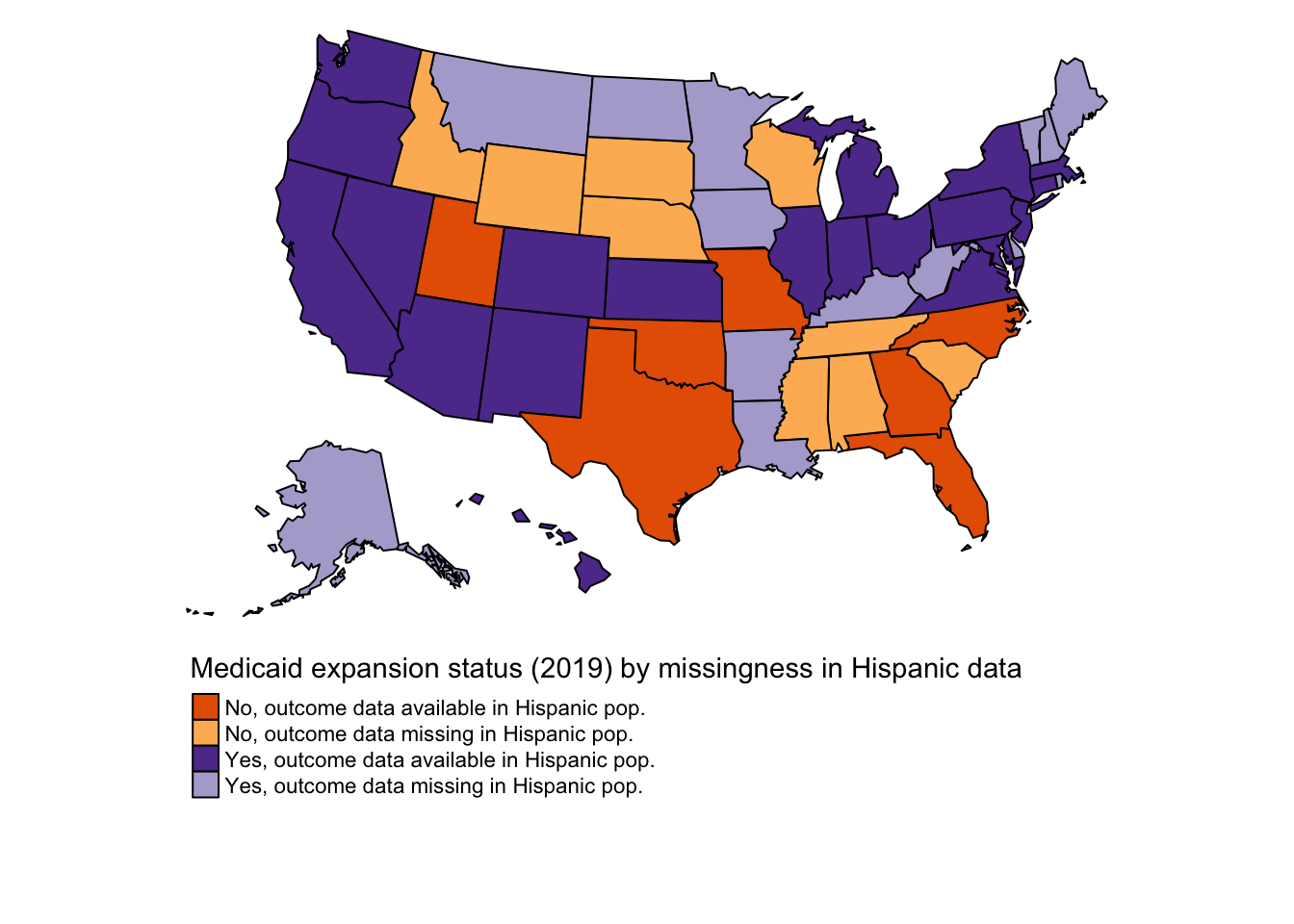
2.1.2 Hispanic population
| treated | n |
|---|---|
| 0 | 7 |
| 1 | 20 |
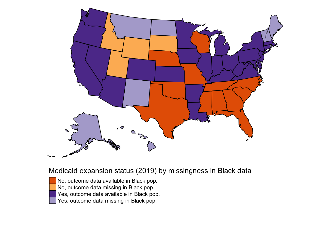
2.1.3 Black population
| treated | n |
|---|---|
| 0 | 12 |
| 1 | 25 |
2.2 Distribution of BRFSS covariates
In this section, I examine the distribution of some of the BRFSS covariates used in the analysis to see if the BRFSS data may be contributing to the instability of the effect estimates.
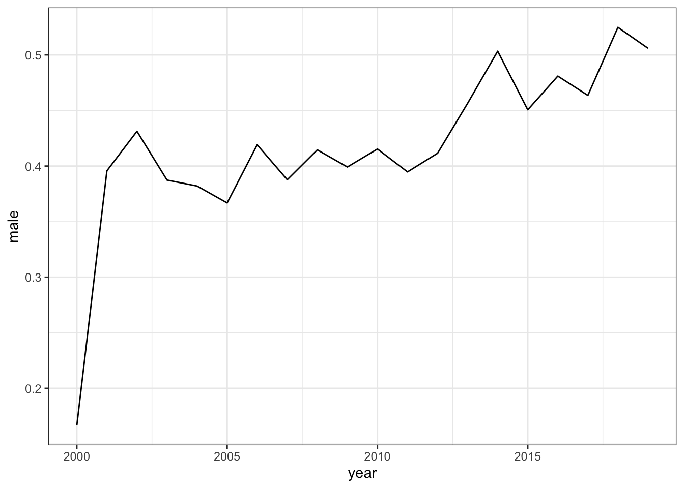
2.2.1 Proportion men
2.2.1.1 All adults aged 45-64
Proportion men among all adults aged 45-64 (dataset name: overall)
##    Min. 1st Qu.  Median    Mean 3rd Qu.    Max.
##  0.3093  0.3957  0.4166  0.4173  0.4400  0.5317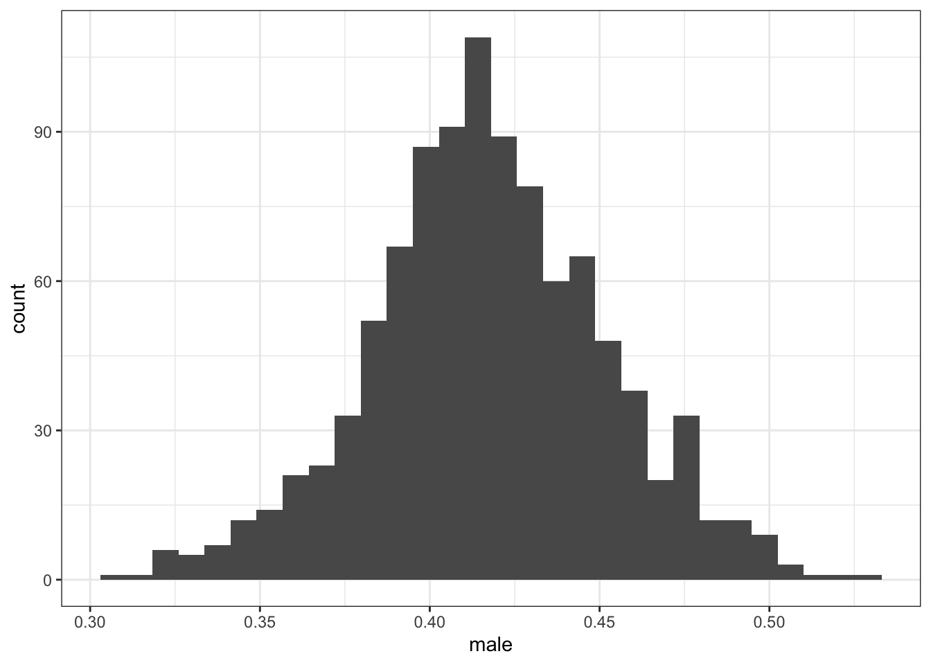
2.2.1.2 Hispanic adults aged 45-64
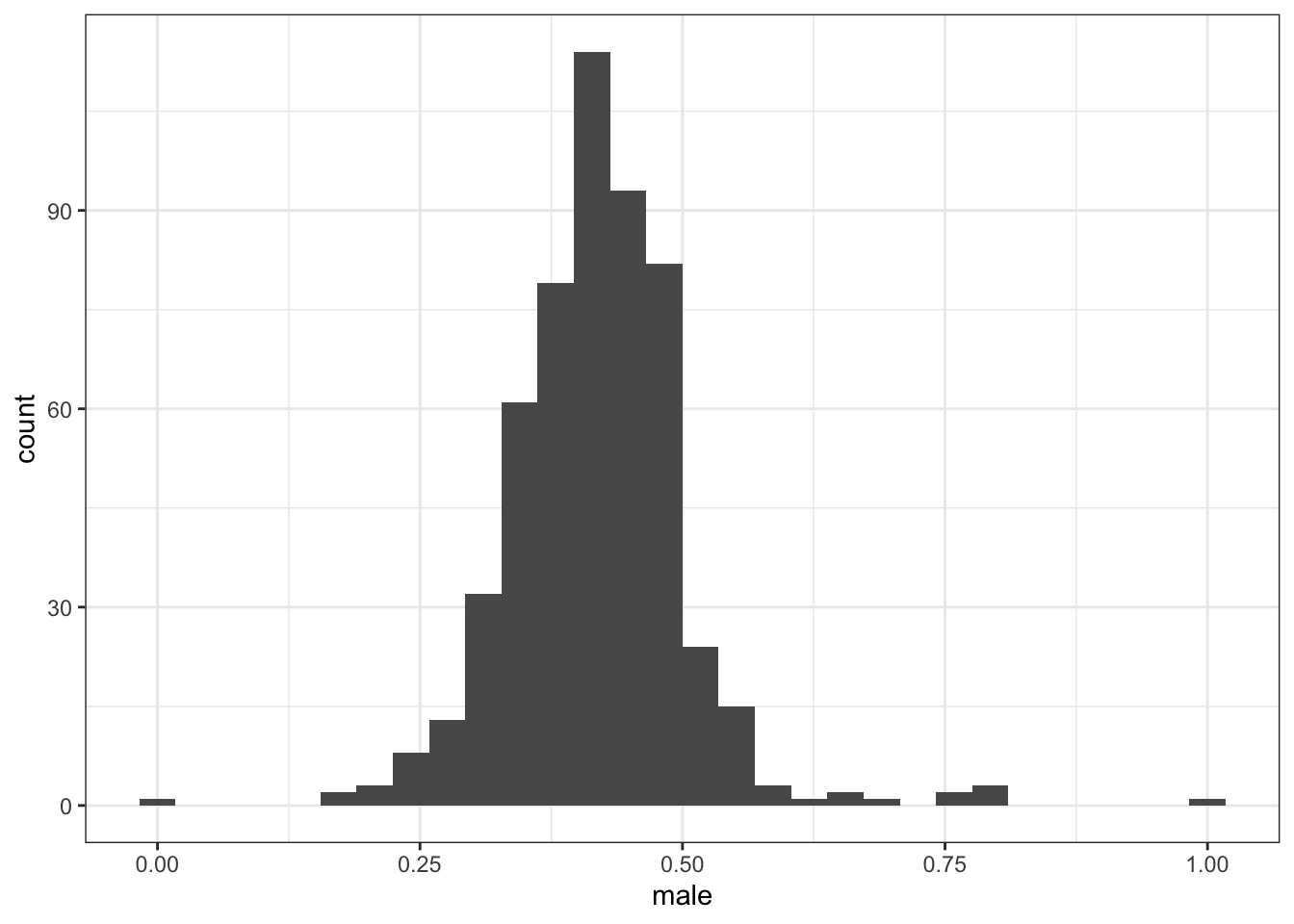
Proportion men among Hispanic adults aged 45-64 (dataset name: hispanic_complete)
Observation: some state-years have 0% or 100% men in this group, which is not plausible, highlighting the fact that BRFSS may not be reliable in such stratified sub-groups.
##    Min. 1st Qu.  Median    Mean 3rd Qu.    Max.
##  0.0000  0.3693  0.4200  0.4188  0.4651  1.0000
In California, most years seem implausibly low.
2.2.1.3 Black adults aged 45-64
Again, the proportion men among Black adults aged 45-64 seems implausible in some state-years.
##    Min. 1st Qu.  Median    Mean 3rd Qu.    Max.
##  0.1579  0.3250  0.3643  0.3761  0.4194  0.7000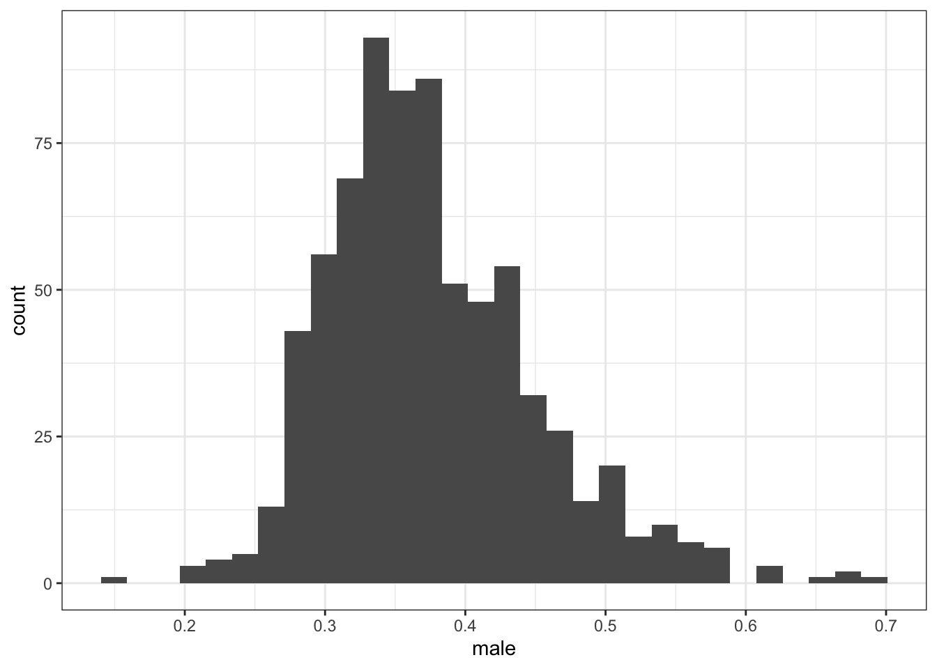
2.2.1.4 White adults aged 45-64
##    Min. 1st Qu.  Median    Mean 3rd Qu.    Max.
##  0.0000  0.3598  0.4196  0.4198  0.4742  1.0000
2.2.2 Low income
Less than $15,000
2.2.2.1 All adults aged 45-64
##    Min. 1st Qu.  Median    Mean 3rd Qu.    Max.
## 0.03898 0.06782 0.08677 0.09121 0.11007 0.19325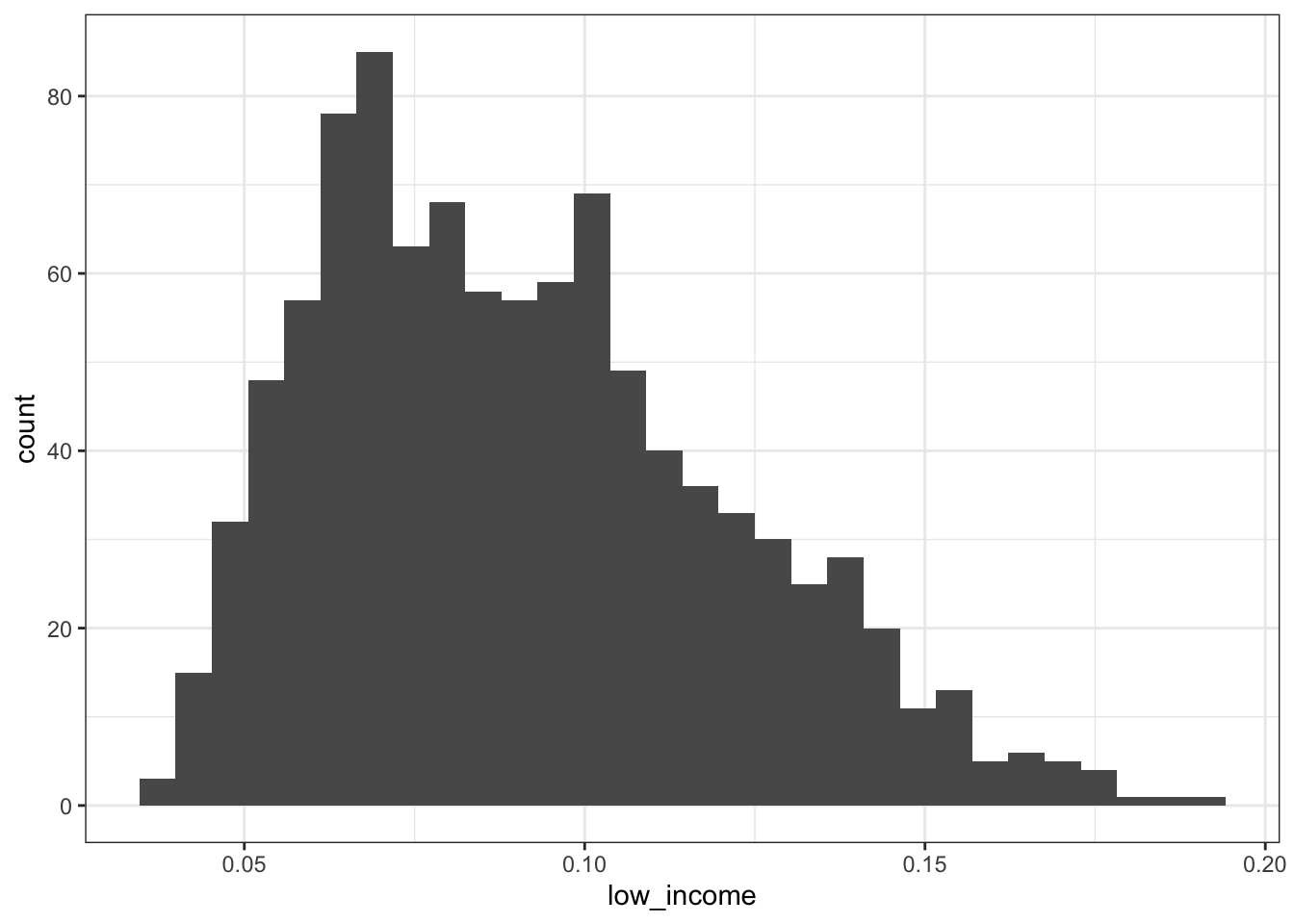
2.2.2.2 Hispanic adults aged 45-64
Again, there are what I would think are some implausible observations (e.g,. 0% or 100% low income in a state-year).
##    Min. 1st Qu.  Median    Mean 3rd Qu.    Max.
##  0.0000  0.1143  0.1533  0.1586  0.1968  1.0000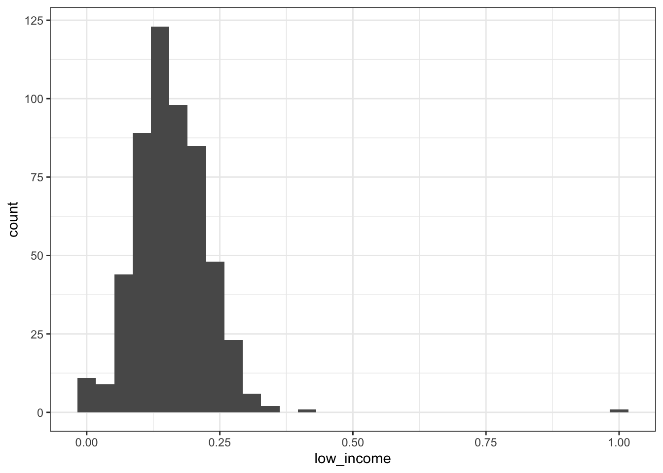
2.2.2.3 Black adults aged 45-64
##    Min. 1st Qu.  Median    Mean 3rd Qu.    Max.
##  0.0000  0.1355  0.1765  0.1784  0.2166  0.5000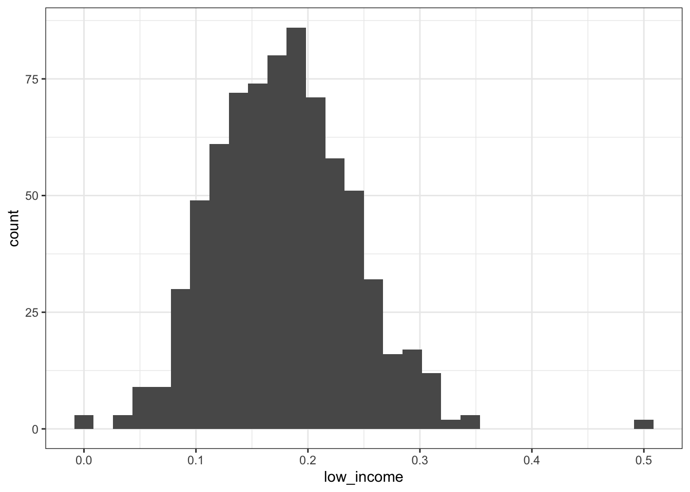
2.2.2.4 White adults aged 45-64
##    Min. 1st Qu.  Median    Mean 3rd Qu.    Max.
## 0.00000 0.09858 0.14219 0.14602 0.19149 1.00000
2.2.3 Low education
No high-school degree
2.2.3.1 All adults aged 45-64
##    Min. 1st Qu.  Median    Mean 3rd Qu.    Max.
## 0.01872 0.04614 0.06653 0.07496 0.09833 0.23663
2.2.3.2 Hispanic adults aged 45-64
##    Min. 1st Qu.  Median    Mean 3rd Qu.    Max.
##  0.0000  0.1780  0.2650  0.2611  0.3486  0.5547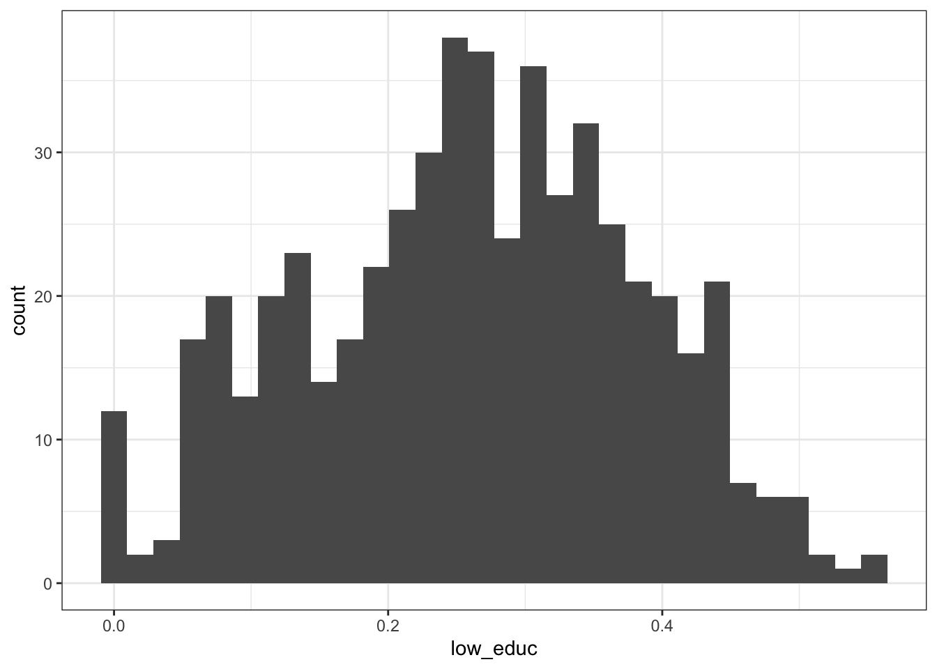
2.2.3.3 Black adults aged 45-64
##    Min. 1st Qu.  Median    Mean 3rd Qu.    Max.
## 0.00000 0.08062 0.11265 0.11936 0.15205 0.50000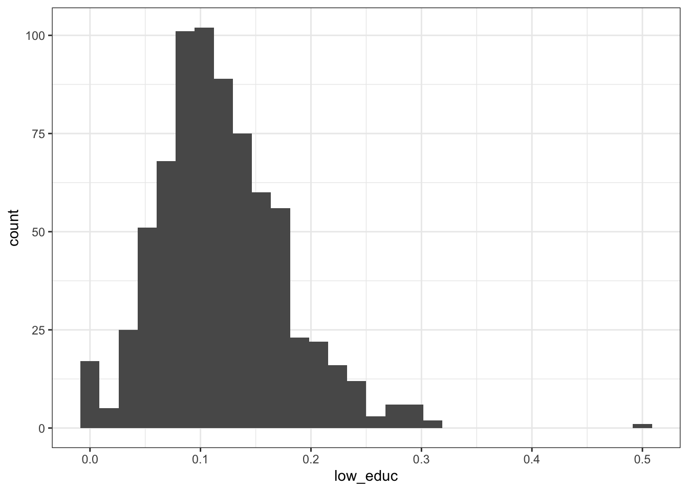
2.2.3.4 White adults aged 45-64
##    Min. 1st Qu.  Median    Mean 3rd Qu.    Max.
##  0.0000  0.1250  0.2268  0.2318  0.3333  0.6400
2.2.4 Married
2.2.4.1 All adults aged 45-64
##    Min. 1st Qu.  Median    Mean 3rd Qu.    Max.
##  0.5029  0.5849  0.6104  0.6137  0.6385  0.7633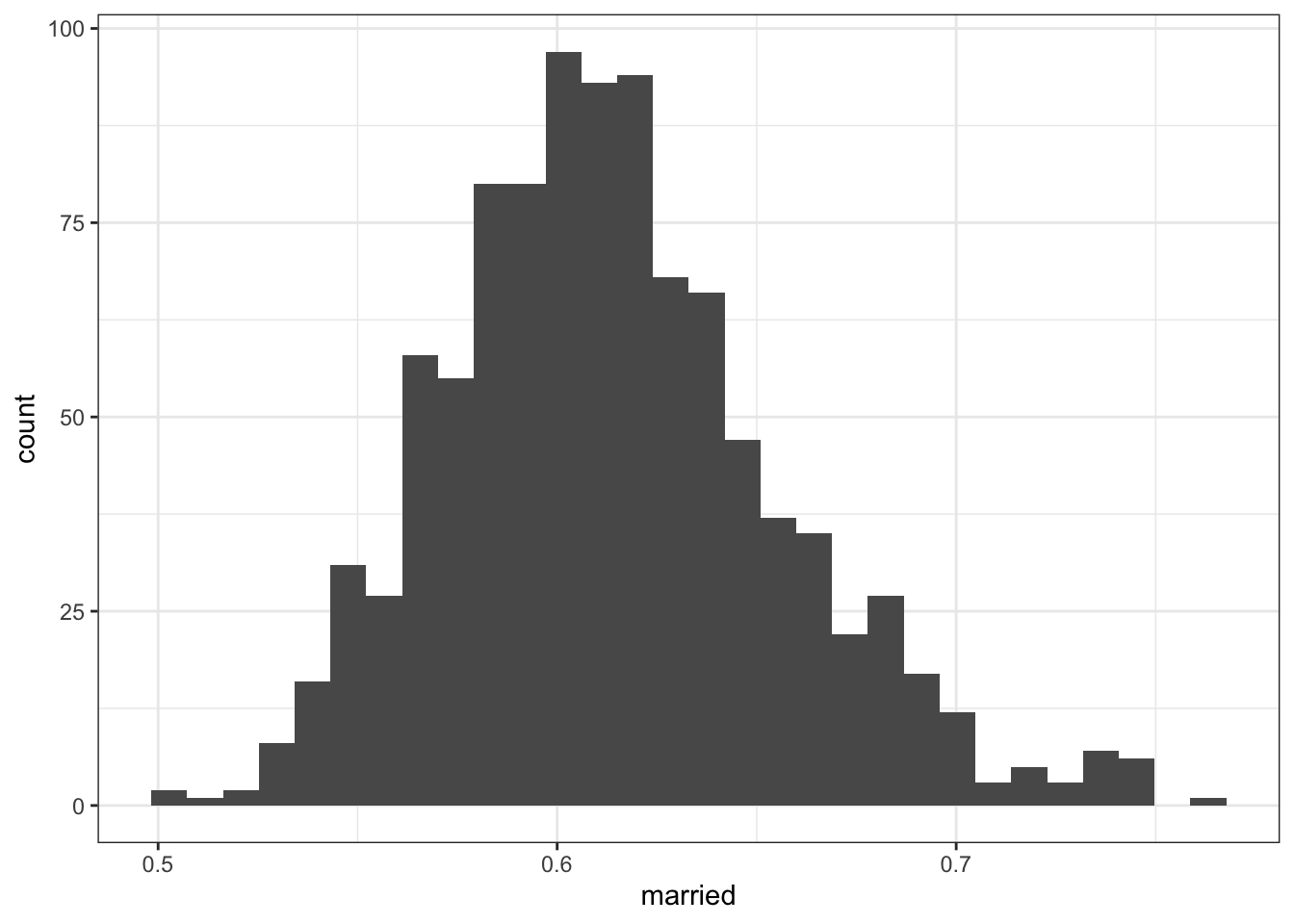
2.2.4.2 Hispanic adults aged 45-64
##    Min. 1st Qu.  Median    Mean 3rd Qu.    Max.
##  0.0000  0.5245  0.5869  0.5759  0.6317  1.0000
2.2.4.3 Black adults aged 45-64
##    Min. 1st Qu.  Median    Mean 3rd Qu.    Max.
##  0.0000  0.3279  0.3735  0.3708  0.4106  0.6111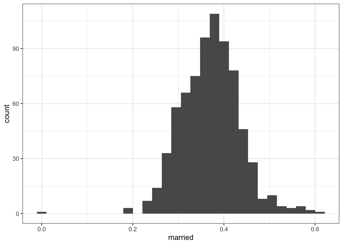
2.2.4.4 White adults aged 45-64
##    Min. 1st Qu.  Median    Mean 3rd Qu.    Max.
##  0.0000  0.5226  0.5890  0.5810  0.6429  1.0000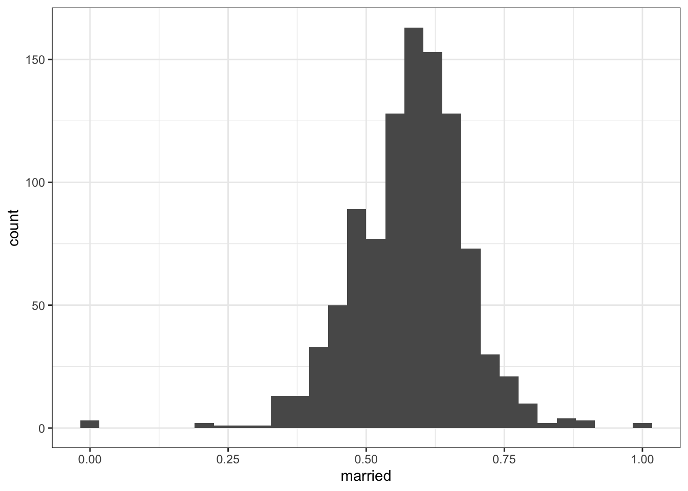
2.2.5 Political orientation and considering an alternative measure
In Nianogo et al.’s Table 1, they present the measure of political-party affiliation in 2014. The below replicates those values, where 0=Republican, 1=Democrat, and 2=Split.
| party | n | n_total | prop |
|---|---|---|---|
| 0 | 24 | 50 | 0.48 |
| 1 | 13 | 50 | 0.26 |
| 2 | 13 | 50 | 0.26 |
To facilitate interpretation, this variable in 2016 is mapped here:
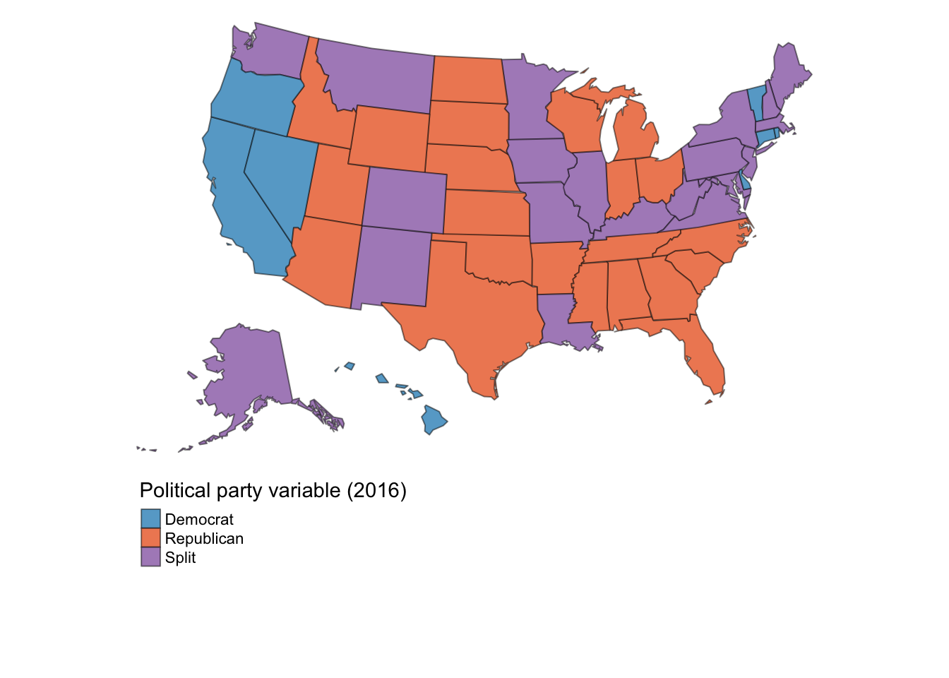
These values struck me as somewhat odd. For one, it appears a given state-year receives a value of either Republican, Democrat, or split, raising the question of within-state variability in the measure. Second, given the polarization and parity of party politics in the United States, I would expect the values corresponding to Republican (0) and Democrat (1) to be about the same and for both to be nearer to 50%.
A simpler and more stable (in terms of sampling variability) measure for the state’s political environment might be the popular-vote share from presidential elections. Those data are available here:
https://dataverse.harvard.edu/dataset.xhtml?persistentId=doi:10.7910/DVN/42MVDX
In this script, I’ve loaded popular-vote data from presidential elections.
source(here("scripts", "read-wrangle-data-pres-election.R"))In analyses as presented in Scenarios 2-5 in the main text, I applied the vote share from the most recent election if the year wasn’t an election year. For example, 2014 received 2012’s popular-vote data.
3 Using state-year effect estimates to calculate various summary measures
In this section, I show how state-year effect estimates generated by the gsynth() function can be used to calculate summary measures of effect. Specifically, in this section, I populate some values corresponding to Scenarios 4 and 5 in the main text’s table.
Code that generates other results can be found here: gsynth-nianogo-et-al/scripts/gsynth-analyses-to-post.R
3.1 Load the data
source(here("scripts", "read-wrangle-data-acs.R"))
source(here("scripts", "read-wrangle-data-pres-election.R"))
source(here("scripts", "read-wrangle-data-nianogo-et-al.R"))
3.2 Run the gsynth function
Here, I will summarize effects estimated by the MC-NNM estimator as presented in Scenarios 4 and 5 of the table in the text.
For more information on the syntax of the gsynth() function, please see:
https://yiqingxu.org/packages/gsynth/articles/tutorial.html#matrix-completion
gsynth_out_overall_sub_pol_mc_nnm=gsynth(
  #syntax: outcome ~ treatment indicator+ covariates
  cvd_death_rate ~ treatedpost +
    primarycare_rate +
    cardio_rate +
    population_overall +
    low_educ_overall +
    married_overall+
    employed_for_wages_overall +
    vote_share_dem+#popular vote data
    low_income_overall +
    male_overall +
    race_nonwhite_overall
  ,

  #dataset in which the effects are estimated
  data = overall_covars_alt,
  estimator = "mc", #the MC-NNM estimator
  #      EM = F, #
  index = c("state_id","year"), #time-unit

  #non-parametric bootstrap if MC-NNM estimator used
  #inference = "parametric",
  se = TRUE,

  #perform a cross-validation procedure to
  #determine the number of unobserved factors
  CV = TRUE,

  #the range of possible numbers of unobserved factors
  r = c(0, 5), #
  seed = 123, #arbitrary seed so same results every time
  nboots = 2000, #number of bootstrap reps
  force = "two-way",
  parallel = TRUE
)
3.3 Examine summary output returned by the gsynth function
3.3.1 Average treatment effect with confidence intervals
Return the average (unweighted) difference effect over all treated state-years and the corresponding standard error and confidence intervals.
gsynth_out_overall_sub_pol_mc_nnm$est.avg## Estimate S.E. CI.lower CI.upper p.value
## ATT.avg -2.118079 2.163304 -6.358078 2.121919 0.3275332These confidence intervals are calculated by adding 1.96SE and -1.96SE to either side of the estimate.
#qnorm(.975)#return the exact value
#Estimate
gsynth_out_overall_sub_pol_mc_nnm$est.avg[1]
## [1] -2.118079#Upper limit
gsynth_out_overall_sub_pol_mc_nnm$est.avg[1]+
gsynth_out_overall_sub_pol_mc_nnm$est.avg[2]*1.959964## [1] 2.121919#Lower limit
gsynth_out_overall_sub_pol_mc_nnm$est.avg[1]-
gsynth_out_overall_sub_pol_mc_nnm$est.avg[2]*1.959964## [1] -6.3580783.3.2 Average treatment effect - point estimate only
Another way to return the point estimate for the average treatment effect (without the confidence intervals) is by gsynth_object$att.avg.
gsynth_out_overall_sub_pol_mc_nnm$att.avg## [1] -2.1180793.3.3 Average treatment effect at each time point
The average treatment effect at each time point can be returned by gsynth_object$att. These effect estimates are summarized by time over units where time is indexed from the treatment period for that unit such that the first treated time point is time 1. By the numbering system below, time 0 is the latest time point of the pre-treatment period.
gsynth_out_overall_sub_pol_mc_nnm$att## -13 -12 -11 -10 -9 -8
## -0.26992263 0.38732901 0.26348340 -0.79655792 -1.01552488 0.23192784
## -7 -6 -5 -4 -3 -2
## 0.08756312 0.14899219 0.23311709 -0.07675195 -0.03369085 0.30835163
## -1 0 1 2 3 4
## 0.40214995 0.14395025 -3.94572630 -4.90217808 -0.48894728 -1.83082518
## 5 6
## -1.53387942 0.562690213.4 Calculate unweighted average difference effect by summarizing effect estimates over treated state-years
3.4.1 Return effect estimates for every treated state-year
Using the effect estimates for every treated state-year, we can replicate the summary difference effects presented above. Effect estimates for every treated state-year are returned by gsynth_objecct$eff.
Here are the difference effects for all state-years. Note that “effects” are estimated for all state-years in the treated states, including pre-treatment years. Pre-treatment effects are not really effects but are the pre-treatment prediction error for treated units: the difference between the observed and predicted counterfactual outcomes before treatment.
gsynth_out_overall_sub_pol_mc_nnm$eff## 2 4 5 6 8 9
## 2000 -2.8549609 0.9254919 -6.56021258 -6.3914770 -2.9607249 5.01758412
## 2001 5.8785560 -2.8025061 -3.46542138 -9.7262748 -10.6700147 1.56284433
## 2002 -0.3513856 3.3130764 5.35241334 -4.2376838 3.4085189 3.31272662
## 2003 -0.3155085 -3.1909703 -9.84283260 2.9835159 -1.1003219 -1.01984959
## 2004 0.5178832 1.2243677 -2.37844455 0.3360901 0.1558620 -0.15402197
## 2005 -5.3910471 2.8557760 0.05381347 0.1484376 -0.5027154 -2.92327032
## 2006 -9.3061276 3.6482257 5.60159505 6.3278789 0.8159762 -4.80527797
## 2007 -13.9966886 2.6698943 -0.12056547 5.3221665 1.3100673 -1.99285818
## 2008 -8.0616089 -3.8467589 5.45840980 -0.2389340 1.7882295 -0.05959601
## 2009 2.2731099 -3.1360315 -4.39773648 1.2113080 5.3525481 0.83235292
## 2010 9.6699464 -4.9302006 1.99157065 1.4377013 -0.4254949 0.93916143
## 2011 4.1806033 1.5230066 6.41778331 0.6398288 3.8678738 -1.52598728
## 2012 6.6324375 2.0246665 5.80748351 4.5018306 3.5084971 5.70294337
## 2013 1.1994690 -0.4073624 -2.26575154 -1.2320234 -2.7471547 -4.53157237
## 2014 12.4764326 -10.2414970 16.40508485 -8.8986156 -0.3509733 -13.46949116
## 2015 11.7806796 -5.9121541 4.40407449 -10.7073366 -2.7536341 -15.30211467
## 2016 10.6629440 2.5407575 14.36990400 -0.6185028 5.6350307 -15.82618933
## 2017 2.7299284 -4.5502136 20.27686278 -3.7604160 -3.9764594 -14.49889136
## 2018 11.5267968 -5.8068421 13.01575069 -4.0113799 -8.7816937 -9.97251318
## 2019 14.0531558 -5.9749003 28.88296298 -4.6492172 -0.4304725 -11.75555220
## 10 15 17 18 19 20
## 2000 -1.81602305 8.0833229 1.9257576 2.3235016 0.1176644 -5.555199395
## 2001 2.13907177 -5.0601838 3.6297837 -2.6650165 -4.8037043 2.217920042
## 2002 -4.35112520 4.3777023 2.1085935 -3.9036759 -7.6005317 -0.915802086
## 2003 -7.92495992 -3.9467320 0.1489462 0.6781281 2.6342882 -0.006407251
## 2004 2.01941293 -0.6863185 0.2391470 4.0858052 -3.3363742 5.469241138
## 2005 -0.45835661 1.6764130 0.6290714 -2.2168794 -1.1991227 3.413243076
## 2006 4.73311789 -0.9313507 -4.2223637 -0.4899900 2.9689752 -0.978106611
## 2007 4.08137468 -9.6010019 -1.3708982 -1.2385030 -1.1254830 -3.807699360
## 2008 8.67188119 2.5259067 3.4691970 0.5785341 -2.2654531 -1.413289722
## 2009 3.44429572 1.4708106 -0.4549505 -2.8616421 1.2561041 -2.850611758
## 2010 0.07237734 -4.9620191 -0.1246502 2.3606650 5.7387897 0.746911783
## 2011 -12.91829889 1.4193114 -0.1147696 1.4696709 1.1421687 1.697238737
## 2012 -6.88068309 1.8411968 -4.1509112 4.8162724 2.7783652 4.608116170
## 2013 7.89468907 4.2960914 -2.5491895 0.7139686 4.6177348 -1.502840268
## 2014 -22.89346887 19.0004806 -11.6410006 -3.3863784 -10.4195965 5.991426220
## 2015 -22.89838332 9.4663920 -14.7722243 -8.2851715 -15.3251365 7.786098766
## 2016 -16.42311988 -12.5374204 -11.3011604 2.3463428 1.2881646 9.341081057
## 2017 -11.29206388 8.4828745 -16.6572568 -2.0741844 -0.6877451 5.604985932
## 2018 -21.13442854 4.5800173 -9.1374801 0.3032116 0.9905305 9.965214467
## 2019 -23.44436702 5.6359251 -13.4046862 1.3658028 19.8335289 6.429658030
## 21 22 23 24 25 26
## 2000 -4.6294111 -1.7437083 0.07570525 2.7204380 -0.6990843 -0.0161745
## 2001 6.4119219 2.6067579 6.69923992 0.6281304 -0.4088048 -3.3504597
## 2002 -5.0860523 -6.1868444 -6.02419187 -2.9893821 2.9089778 -2.5980492
## 2003 0.5004803 3.6138866 -1.15556061 -1.6482439 6.5289678 1.5007905
## 2004 -1.9404038 -1.1781295 -5.84272521 4.6644422 4.4017002 -2.8865029
## 2005 0.5737142 2.4002428 3.15175303 0.2256716 -3.3073082 4.1748908
## 2006 -0.2055802 2.2460686 9.59173002 0.1218915 -2.1117501 -2.9027444
## 2007 -4.0766510 0.9936110 3.68216281 1.3875399 2.9845796 3.3115265
## 2008 -3.2261717 8.1203126 -0.75057774 -3.0707603 -1.3134053 0.6602714
## 2009 -0.8405247 -0.0926782 -10.05108079 4.9282587 0.4090805 -1.0117059
## 2010 1.3752575 -3.4818804 -5.42439483 2.9718065 -2.5460516 -0.6252006
## 2011 2.3199656 -12.9166318 5.97492694 -4.9875114 -1.4695736 5.0311348
## 2012 8.8105395 0.5373354 -0.36686424 -3.5569524 -1.1951496 -0.6589605
## 2013 1.6694429 1.7842381 -3.20559413 -2.3161417 -4.0163692 -0.8177121
## 2014 6.8212288 6.7992718 -1.26734251 -12.1052757 -10.2694142 -3.7923500
## 2015 12.7207553 -3.9471131 8.21634494 -7.1830097 -12.1394040 -9.1702556
## 2016 23.5383831 3.6295946 1.36876148 -5.0372080 -10.0868757 3.8551289
## 2017 15.5653180 6.7371183 -1.84861304 -10.3177240 -11.1426868 -6.6989052
## 2018 16.1854734 -4.3213319 -3.00867593 -5.0233898 -12.5516589 -7.1359537
## 2019 19.4853982 -2.7256552 -6.19037815 -8.6562222 -10.0813651 -13.5660754
## 27 30 32 33 34 35
## 2000 -4.0048696 -1.3426304 -4.65485271 1.297806 3.49322602 -8.7826231
## 2001 -0.1704084 -1.0810075 2.14520702 4.990289 1.89685211 -1.1569962
## 2002 -2.0120038 4.5521697 -4.44486600 6.015901 1.83996172 3.6758075
## 2003 -4.9673122 6.4480646 -1.11728952 -10.111013 0.70623219 -5.3882315
## 2004 0.1339679 -10.5633307 1.44698982 -5.876708 -1.34815685 -6.9289465
## 2005 2.9537924 -4.9570906 14.73236650 -4.786283 2.87606329 2.2905988
## 2006 -1.6440201 -6.6824458 7.34860789 6.833601 -0.05237921 -3.2057401
## 2007 1.0162709 7.9289953 -8.30998500 4.348816 -3.12345705 3.5031667
## 2008 0.4591471 1.6399859 -5.22629959 -4.437997 -1.47227800 0.7100342
## 2009 1.8882641 1.3506144 7.05149787 3.132310 -12.37021673 6.4353284
## 2010 0.1269997 1.1665361 -4.22738418 -6.564625 6.54540853 4.3688844
## 2011 1.7030661 2.4417498 -0.99729630 -1.901203 1.24024958 4.3837180
## 2012 4.4449333 -0.2856542 -4.29067883 1.298751 1.08499560 -5.0201027
## 2013 1.0497289 2.2230876 -0.07108479 5.590018 -1.33348534 6.6105782
## 2014 -4.1888925 -5.1417667 -8.98697513 -11.272948 -7.67655067 3.1359613
## 2015 -8.0823884 2.2432412 -2.12211379 -10.839888 -12.53180244 -5.7178546
## 2016 -2.6465417 -4.0264410 0.90474778 4.272769 -8.07086934 21.6165209
## 2017 0.9229848 -3.4163772 -12.80839412 1.648234 -7.25530872 7.0654661
## 2018 -0.5146687 14.1233195 -15.25640221 10.693277 -6.43962457 6.6653689
## 2019 -2.9910751 9.3273563 -7.47229206 6.713150 -9.11903698 23.2141307
## 36 38 39 41 42 44
## 2000 1.4980350 -0.7849287 2.72070183 -2.74410407 4.7260493 -8.7893744
## 2001 2.2277692 8.5343622 2.15891822 0.19279412 -0.2558283 0.3017889
## 2002 3.3868805 3.7200846 0.16329797 3.17342622 0.2748056 10.1671798
## 2003 -1.8994282 -0.9878865 -5.94840869 3.99131946 0.5119358 1.4843829
## 2004 -0.4386471 -2.9003550 1.14380012 -0.64099565 -1.2416699 5.9246401
## 2005 -4.0692782 -13.8914755 0.09257012 -1.01699490 3.0248903 12.5212797
## 2006 1.3508449 2.6358211 0.10715142 0.04729964 -0.2894381 -12.6922983
## 2007 1.7391272 -1.1568271 -0.47011710 4.96863701 1.4617728 0.9401307
## 2008 3.1639697 1.8887027 5.11960520 -1.10792700 1.3787021 2.6453143
## 2009 2.7955844 5.2327818 -11.23860745 2.46069932 1.5827381 -1.1426075
## 2010 0.9548831 1.2728407 2.39731545 -6.91189540 0.4103455 -9.1348055
## 2011 -2.8668582 -9.2538635 -1.12805468 -2.02654500 3.7307358 1.7752254
## 2012 -2.1615826 4.3282893 2.08242672 -0.31258942 -5.8830510 -3.3541590
## 2013 -6.7585549 1.8432708 2.26863503 -0.39629928 -2.9168291 0.7092182
## 2014 -11.7479432 11.0310816 -3.72879683 -8.85201412 -7.9378003 -8.1255893
## 2015 -15.8285250 1.5682665 -5.34896552 -6.75804086 -8.7787923 -13.1770728
## 2016 -8.9845593 -6.9688493 1.43973387 -7.60298008 -5.1766789 -24.4935331
## 2017 -14.9863614 -3.6408701 1.40894744 -3.58769597 -6.9289439 -15.4903265
## 2018 -13.5788328 -10.1648103 2.92951948 -11.07381110 -4.5559510 -6.9201632
## 2019 -13.1826499 9.3520661 3.44603107 -8.14339630 -5.8061284 -12.2986461
## 50 51 53 54
## 2000 9.3334980 3.52262819 -2.51466703 7.082314
## 2001 -7.5470297 3.76949417 0.68184390 7.907938
## 2002 -6.5770902 0.16162444 -1.02277580 1.651880
## 2003 -1.9011750 -3.77901751 4.39397664 4.535699
## 2004 -5.1006728 5.14870161 2.07462053 -13.245792
## 2005 -5.2770927 3.03572786 -0.67048990 3.057515
## 2006 0.6724051 -0.96986954 -4.55335693 -2.637055
## 2007 -0.2832529 -0.59788780 2.21108611 5.607797
## 2008 5.8980325 4.45490136 4.17312190 -4.072115
## 2009 0.3522267 3.17070597 -2.44856779 -6.761062
## 2010 4.8594316 0.30006093 1.47493946 -7.671514
## 2011 6.8838652 -1.25602873 -2.04069510 2.261032
## 2012 -7.2772523 0.31565145 -1.85751154 3.007931
## 2013 5.3846361 -2.42812390 0.02122725 -2.535492
## 2014 2.0799530 -4.90912715 -3.90396235 -10.993697
## 2015 11.1466987 -8.14496292 -9.25678926 -9.288240
## 2016 25.5202676 -1.53260149 -4.13516149 1.235381
## 2017 12.7525180 -0.24683486 -3.50708670 -1.331951
## 2018 15.5950791 -0.01963506 -3.36883864 14.623048
## 2019 25.5960077 -3.19034963 -3.27040641 15.0441383.4.2 Wrangle state-year effect estimates in easier-to-read form
Do some data wrangling to the effect estimates to summarize them.
Notes on my naming conventions for the object:
- tib: for tibble
- diff_eff_by_state_year: difference effects by state-year
- mc_nnm: to indicate which gsynth model it corresponds to
Also note that these results are among the total population (“overall”), not a particular demographic subgroup.
tib_diff_eff_by_state_year_mc_nnm=gsynth_out_overall_sub_pol_mc_nnm$eff %>%
  as_tibble() %>% #Convert to tibble
  mutate(year=row_number()+1999)  %>% #Add 1999 to row number to calculate year
  dplyr::select(year,everything()) %>%
  pivot_longer(cols=-year) %>%  #make the dataset long-form
  #Rename some of the columns
  rename(
    state_id = name,
    diff_pt = value #estimated difference effect
    ) %>%
  mutate(state_id=as.numeric(state_id)) #make sure state_id is numeric

tib_diff_eff_by_state_year_mc_nnm
## # A tibble: 680 × 3
## year state_id diff_pt
## <dbl> <dbl> <dbl>
## 1 2000 2 -2.85
## 2 2000 4 0.925
## 3 2000 5 -6.56
## 4 2000 6 -6.39
## 5 2000 8 -2.96
## 6 2000 9 5.02
## 7 2000 10 -1.82
## 8 2000 15 8.08
## 9 2000 17 1.93
## 10 2000 18 2.32
## # ℹ 670 more rowsBefore we summarize these difference effect estimates, we can link in the treatment indicator so that we know whether the difference effects are during the post-treatment period. The treatment indicator is obtained by calling gsynth_object$D.tr.
(The letter D is conventionally used in the econometrics literature to denote the treatment status.)
tib_treatedpost =gsynth_out_overall_sub_pol_mc_nnm$D.tr %>%
  as_tibble() %>%
  mutate(year=row_number()+1999) %>%
  dplyr::select(year,everything()) %>%
  pivot_longer(cols=-year) %>%
  rename(
    state_id = name,
    treatedpost = value) %>%
  mutate(state_id=as.numeric(state_id))

tib_treatedpost
## # A tibble: 680 × 3
## year state_id treatedpost
## <dbl> <dbl> <dbl>
## 1 2000 2 0
## 2 2000 4 0
## 3 2000 5 0
## 4 2000 6 0
## 5 2000 8 0
## 6 2000 9 0
## 7 2000 10 0
## 8 2000 15 0
## 9 2000 17 0
## 10 2000 18 0
## # ℹ 670 more rows3.4.3 Calculate unweighted average difference effect
Now we can link those two together to summarize the difference effects over the post-treatment period (which varies by state). It should match the average treatment effect obtained above.
diff_pt_mean_mc_nnm=tib_diff_eff_by_state_year_mc_nnm %>%
  #Link the treatment indicator to the difference effects by state-year
  left_join(tib_treatedpost,by=c("state_id","year")) %>%
  group_by(treatedpost) %>%
  #take the simple mean by treatment indicator
  summarise(
    diff_pt_mean=mean(diff_pt,na.rm=T)
  )

diff_pt_mean_mc_nnm
## # A tibble: 2 × 2
## treatedpost diff_pt_mean
## <dbl> <dbl>
## 1 0 0.0116
## 2 1 -2.12The average difference effect post-treatment indeed matches the value returned by gsynth_object$att.avg, which demonstrates that the average treatment effect returned by the gsynth’s default output is the unweighted average over treated state-years.
gsynth_out_overall_sub_pol_mc_nnm$att.avg## [1] -2.1180793.4.4 Calculate 95% confidence intervals for the unweighted average difference effect using the bootstrap replicates.
First, return bootstrapped effect estimates for every state-year in every replicate by calling gsynth_object$eff.boot.
tib_eff_boot_mc_nnm=gsynth_out_overall_sub_pol_mc_nnm$eff.boot %>%
  #converting to tibble makes the data such that there
  #are 20 rows and 6,800 columns, each with information
  #containing the bootstrapped effect estimates.
  #We need to organize the data such that each row
  #represents a unit-month-bootstrap replicate
  as_tibble() %>%
  #Note each row represents the time variable.
  #The observation period begins in 2000, so
  #we should add 1999 to the row number to get the first obs
  #to be 2000
  mutate(year=row_number()+1999) %>%
  #make year the left-most variable to make it easier to see
  dplyr::select(year,everything()) %>%
  #now make the data long form
  pivot_longer(cols=-year) %>%
  #we now have three variables: year, name, and value.
  #the "name" variable contains the state id and the bootstrap
  #replicate. We need to separate these two values into separate variables.
  #We can use separate_wider_delim() for this from tidyr
  separate_wider_delim(name,names=c("state_id","boot_rep"), ".") %>%
  #make the state_id and boot_rep (boot replication) variables numeric
  mutate(
    state_id=as.numeric(state_id),
    boot_rep_char=str_sub(boot_rep, 5,11),#5 to 11 in case lots of digits
    boot_rep=as.numeric(boot_rep_char)
  ) %>%
  dplyr::select(-boot_rep_char) %>%   #drop vars not needed
  #note the difference-based effect estimate is stored in "value"
  #let's call it diff_boot
  rename(diff_boot =value)

tib_eff_boot_mc_nnm
## # A tibble: 1,360,000 × 4
## year state_id boot_rep diff_boot
## <dbl> <dbl> <dbl> <dbl>
## 1 2000 2 1 -1.07
## 2 2000 4 1 9.70
## 3 2000 5 1 3.89
## 4 2000 6 1 0.654
## 5 2000 8 1 3.89
## 6 2000 9 1 -6.57
## 7 2000 10 1 -4.80
## 8 2000 15 1 -2.65
## 9 2000 17 1 3.12
## 10 2000 18 1 -3.37
## # ℹ 1,359,990 more rowsPerform some checks on this dataset. The number of rows should equal the number of bootstrap replicates times the number of years times the number of states.
We specified 2,000 boostrap replicates in the gsynth() function above.
There are 34 states included in the analysis.
n_distinct(tib_eff_boot_mc_nnm$state_id)## [1] 34And there are 20 years included in the analysis.
n_distinct(tib_eff_boot_mc_nnm$year)## [1] 20So the number of rows should equal
2000*n_distinct(tib_eff_boot_mc_nnm$state_id)*n_distinct(tib_eff_boot_mc_nnm$year)## [1] 1360000Does it?
nrow(tib_eff_boot_mc_nnm)## [1] 1360000Yes.
Now we can summarize these bootstrapped difference effects to calculate 95% confidence intervals. The process for this is to first calculate average treatment effects for each of the 2,000 bootstrap replicates and then find the 2.5th and 97.5th percentiles over those replicates.
diff_boot_mean_mc_nnm=tib_eff_boot_mc_nnm %>%
  #First calculate average treatment effects for each replicate
  left_join(tib_treatedpost,by=c("state_id","year")) %>%
  group_by(boot_rep, treatedpost) %>%
  summarise(
    diff_boot_mean=mean(diff_boot,na.rm=T)
  ) %>%
  ungroup() %>%
  #We can filter to treatedpost==1 - no need for the pre-treatment effects
  filter(treatedpost==1) %>%
  #Now find the 2.5th and 97.5th value
  group_by(treatedpost) %>%
  summarise(
    diff_pt_ll=quantile(diff_boot_mean, probs=0.025, na.rm=TRUE),
    diff_pt_ul=quantile(diff_boot_mean,probs=.975,na.rm=TRUE)
  )
## `summarise()` has grouped output by 'boot_rep'. You can override using the
## `.groups` argument.diff_boot_mean_mc_nnm## # A tibble: 1 × 3
## treatedpost diff_pt_ll diff_pt_ul
## <dbl> <dbl> <dbl>
## 1 1 -6.42 1.85Those are the confidence intervals corresponding to the overall estimate in Scenario 4 in the table in the main text.
3.5 Calculate unweighted average ratio effects
3.5.1 Point estimates
Ratio effects can also be calculated using this method by comparing the predicted counterfactual outcomes in the treated (gsynth_object$Y.ct) with the actual outcomes (gsynth_object$Y.tr).
#actual outcome in treated
tib_y_tr_mc_nnm=gsynth_out_overall_sub_pol_mc_nnm$Y.tr %>%
  as_tibble() %>%
  mutate(year=row_number()+1999) %>%
  dplyr::select(year,everything()) %>%
  pivot_longer(cols=-year) %>%
  rename(
    state_id = name,
    y_tr_pt = value #observed treated value, pt for point estimate
  ) %>%
  mutate(state_id =as.numeric(state_id))


# Counterfactual outcome in treated
tib_y_ct_mc_nnm=gsynth_out_overall_sub_pol_mc_nnm$Y.ct %>%
  as_tibble() %>%
  mutate(year=row_number()+1999) %>%
  dplyr::select(year,everything()) %>%
  pivot_longer(cols=-year) %>%
  rename(
    state_id = name,
    y_ct_pt = value#estimated counterfactual value, pt for point estimate
  ) %>%
  mutate(state_id =as.numeric(state_id))
Link them together with the treatment-status indicator and find differences and ratios
tib_mc_nnm=tib_treatedpost %>%
  left_join(tib_y_tr_mc_nnm,by=c("year","state_id")) %>%
  left_join(tib_y_ct_mc_nnm,by=c("year","state_id")) %>%
  left_join(tib_diff_eff_by_state_year_mc_nnm,by=c("year","state_id")) %>%
  #Check to make sure that the difference calculated
  #by subtracting the observed outcome from the counterfactual outcome
  #is the same as the reported state-year effect estimates.
  #Rename the difference effect reported by .eff
  rename(diff_pt_report=diff_pt) %>%
  #Calculate differences and ratios
  mutate(
      diff_pt=y_tr_pt-y_ct_pt,#difference effect (point estimate)
      ratio_pt=y_tr_pt/y_ct_pt, #Ratio effect (point estimate)

#      As a check, are these the same?
      diff_pt_check=diff_pt_report-diff_pt

  )


tib_mc_nnm
## # A tibble: 680 × 9
## year state_id treatedpost y_tr_pt y_ct_pt diff_pt_report diff_pt ratio_pt
## <dbl> <dbl> <dbl> <dbl> <dbl> <dbl> <dbl> <dbl>
## 1 2000 2 0 155. 158. -2.85 -2.85 0.982
## 2 2000 4 0 173. 172. 0.925 0.925 1.01
## 3 2000 5 0 252. 259. -6.56 -6.56 0.975
## 4 2000 6 0 168. 174. -6.39 -6.39 0.963
## 5 2000 8 0 130 133. -2.96 -2.96 0.978
## 6 2000 9 0 158 153. 5.02 5.02 1.03
## 7 2000 10 0 195. 197. -1.82 -1.82 0.991
## 8 2000 15 0 185. 177. 8.08 8.08 1.05
## 9 2000 17 0 208. 206. 1.93 1.93 1.01
## 10 2000 18 0 214. 212. 2.32 2.32 1.01
## # ℹ 670 more rows
## # ℹ 1 more variable: diff_pt_check <dbl>As a check on these calculations, diff_pt_check should be zero in all observations
summary(tib_mc_nnm$diff_pt_check)## Min. 1st Qu. Median Mean 3rd Qu. Max.
## 0 0 0 0 0 0We can now calculate average ratio effects in the treated over treated state-years. The ratio effect estimand of interest is the mean of the observed outcome in the treated divided by the mean of the countefactual outcome in the treated. In general, the arithmetic mean of ratios is not generally the same as the ratio of arithmetic means, so we should not take the arithmetic mean of the state-year ratio effects, We can find the summary ratio effect by finding the mean of treated counterfactual outcomes in the treated state-years and the mean of observed outcomes in the treated state-years and then taking the ratio of those two means.
ratio_pt_mc_nnm=tib_mc_nnm %>%
  filter(treatedpost==1) %>%
  group_by(treatedpost) %>%
  summarise(
    y_tr_pt_mean=mean(y_tr_pt,na.rm=T),#observed treated value
    y_ct_pt_mean=mean(y_ct_pt,na.rm=T),#counterfactual
  ) %>%
  ungroup() %>%
  mutate(
    ratio_pt_mean=y_tr_pt_mean/y_ct_pt_mean #ratio effect, point estimate
  )

ratio_pt_mc_nnm
## # A tibble: 1 × 4
## treatedpost y_tr_pt_mean y_ct_pt_mean ratio_pt_mean
## <dbl> <dbl> <dbl> <dbl>
## 1 1 144. 146. 0.986This estimated ratio effect of 0.99 corresponds to the reported overall ratio effect for scenario 4 in the table in the main text.
3.5.2 Confidence intervals
As we did for difference effects, we can calculate confidence intervals around this ratio effect by calculating the ratio effect in each bootstrap replicate and then finding the 2.5th and 97.5th percentiles over replicates.
In each replicate, we can calculate the estimated counterfactual outcome by subtracting the bootstrap’s difference effect from the observed outcome.
#We can work from the previous tibble we created corresponding to the difference-based
#bootstrapped effect estimates
ratio_ci_mc_nnm=tib_eff_boot_mc_nnm %>%
  left_join(tib_mc_nnm,by=c("state_id","year")) %>% #link in the data just above
  filter(treatedpost==1) %>% #limit to treated observations
  mutate(
    y_ct_boot=y_tr_pt-diff_boot #counterfactual estimate - bootstrap
  ) %>%
  #now calculate summary ratio effect in each replicate
  group_by(boot_rep, treatedpost) %>%
  summarise(
      y_tr_pt_mean=mean(y_tr_pt,na.rm=T),#observed treated value, mean (doesn't vary by boot rep)
      y_ct_boot_mean=mean(y_ct_boot,na.rm=T)
  ) %>%
  ungroup() %>%
  mutate(
    ratio_boot_mean=y_tr_pt_mean/y_ct_boot_mean
  ) %>%
    #Now return the 95% confidence intervals of the mean bootstrapped
  #difference effect over replicates
  group_by(treatedpost) %>%
  summarise(
      ratio_pt_ll=quantile(ratio_boot_mean, probs=0.025, na.rm=TRUE),
      ratio_pt_ul=quantile(ratio_boot_mean,probs=.975,na.rm=TRUE)
  )
## `summarise()` has grouped output by 'boot_rep'. You can override using the
## `.groups` argument.Ratio effect point estimate
ratio_pt_mc_nnm## # A tibble: 1 × 4
## treatedpost y_tr_pt_mean y_ct_pt_mean ratio_pt_mean
## <dbl> <dbl> <dbl> <dbl>
## 1 1 144. 146. 0.986Ratio effect 95% CI
ratio_ci_mc_nnm## # A tibble: 1 × 3
## treatedpost ratio_pt_ll ratio_pt_ul
## <dbl> <dbl> <dbl>
## 1 1 0.957 1.013.6 Assess model fit before treatment
We can also assess model fit before treatment using the difference-based “effect” estimates before treatment. Before treatment, these differences are not effects but are the pre-treatment prediction error.
In the main text of the table, I used mean absolute error to measure model fit. Mean squared error or root mean squared error could also be used. I calculate these three measures below.
#Let's begin with this tibble, which already contains all of the difference-based
#effect estimates
pre_tx_fit_mc_nnm=tib_mc_nnm %>%
  mutate(
    #The mean absolute error is the mean of the absolute value of the difference-based
    #effect estimates before treatment.
    diff_pt_abs=abs(diff_pt),

    #To calculate mean squared error, we can first square the difference-based effect
    #estimates and then take the mean
    diff_pt_squared=diff_pt**2
  ) %>%
  filter(treatedpost==0) %>% #0 meaning pre-treatment
  group_by(treatedpost) %>%
  summarise(
    diff_pt_abs_mean=mean(diff_pt_abs,na.rm=T),
    diff_pt_squared_mean=mean(diff_pt_squared,na.rm=T)
  ) %>%
  mutate(
      #square root the square error
      diff_pt_root_mean_square=sqrt(diff_pt_squared_mean)
  )
The mean absolute error of 3.3 corresponds to the reported value for scenario 4 in the table in the main text
pre_tx_fit_mc_nnm## # A tibble: 1 × 4
## treatedpost diff_pt_abs_mean diff_pt_squared_mean diff_pt_root_mean_square
## <dbl> <dbl> <dbl> <dbl>
## 1 0 3.32 19.0 4.363.7 Weighted average treatment effects
When considering the overall population-level effect of the policy, it may be desirable to weight states proportional to their share of that total population (or, more precisely, person-time as there is a temporal component). In this section, I calculate a weighted-average treatment effect, weighting each treated state-year’s effect estimate by its share of treated person time.
3.7.1 Exploring weights
The weights for a given state-year are that state-year’s proportion of the total treated person-years among adults aged 45-64 (variable name: prop_of_tot_pop_year). I gathered state-year populations of adults aged 45-64 from the American Community Survey. These scripts have more details on that:
- scripts/read-wrangle-data-acs.R
- scripts/read-wrangle-data-nianogo-et-al.R
Here a histogram of the weights in the treated state-years.
setwd(here("data","data-processed"))
load("state_year_wts_overall.RData")
state_year_wts_overall %>%
  ggplot(aes(prop_of_tot_pop_year))+
  geom_histogram()+
  theme_bw()
## `stat_bin()` using `bins = 30`. Pick better value with `binwidth`.
Each observation in this dataset of weights is a state-year. The weights add up to 1 over treated state-years.
state_year_wts_overall## # A tibble: 187 × 4
## state_id year pop_tot_all_treated_years prop_of_tot_pop_year
## <dbl> <dbl> <dbl> <dbl>
## 1 4 2014 309495338 0.00527
## 2 5 2014 309495338 0.00242
## 3 6 2014 309495338 0.0315
## 4 8 2014 309495338 0.00446
## 5 9 2014 309495338 0.00335
## 6 10 2014 309495338 0.000817
## 7 15 2014 309495338 0.00116
## 8 17 2014 309495338 0.0110
## 9 19 2014 309495338 0.00264
## 10 20 2014 309495338 0.00235
## # ℹ 177 more rowsstate_year_wts_overall %>%
mutate(dummy=1) %>%
group_by(dummy) %>%
summarise(prop_of_tot_pop_year=sum(prop_of_tot_pop_year))## # A tibble: 1 × 2
## dummy prop_of_tot_pop_year
## <dbl> <dbl>
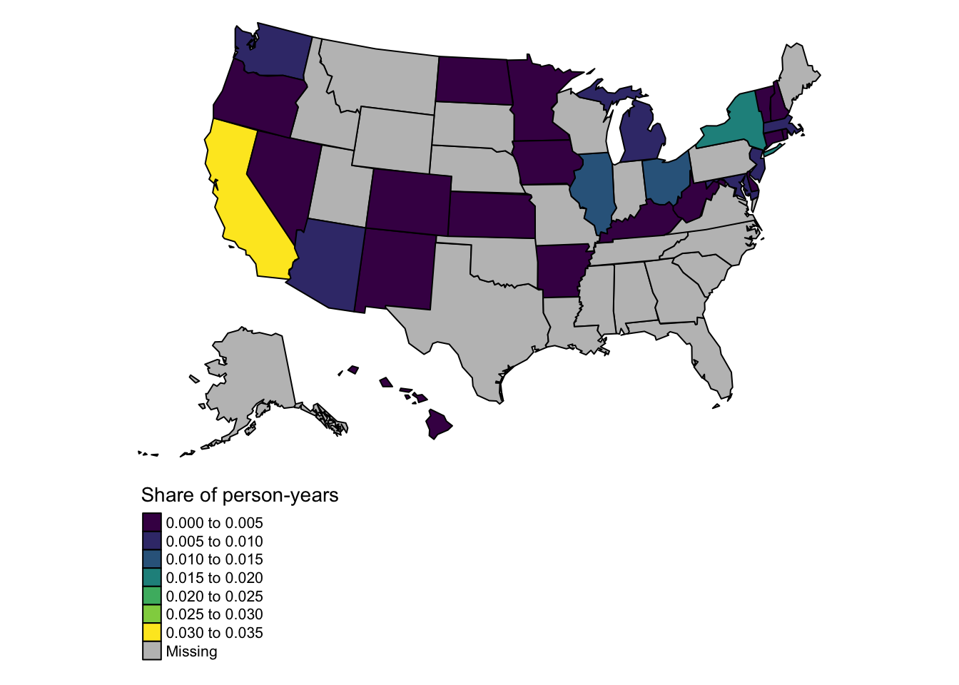
## 1 1 1.00Here’s a map of the weights in 2019. In a given year, they do not sum to 1 because they sum to 1 over all treated state-years.
setwd(here("data","data-processed"))
load("lookup_state_id_state_abb.RData")
state_year_wts_overall_2019=state_year_wts_overall %>%
  filter(year==2019)
lookup_state_abb_geo_simplify_shift_al_hi %>%
  left_join(lookup_state_id_state_abb,by="state_abb") %>%
  left_join(state_year_wts_overall_2019,by="state_id") %>%
  tm_shape()+
  tm_fill(
        "prop_of_tot_pop_year",
        palette =viridis(n=5),
  title="Share of person-years")+
  tm_borders(col="black",alpha=1)+
    tm_layout(
    frame=F,
#    legend.title.size=.5,
    legend.outside=T,
    legend.outside.position="bottom"
    )
The same map in 2014. There are fewer states with non-missing data in this map because fewer states had expanded Medicaid in 2014.
setwd(here("data","data-processed"))
load("lookup_state_id_state_abb.RData")
state_year_wts_overall_2014=state_year_wts_overall %>%
  filter(year==2014)
lookup_state_abb_geo_simplify_shift_al_hi %>%
  left_join(lookup_state_id_state_abb,by="state_abb") %>%
  left_join(state_year_wts_overall_2014,by="state_id") %>%
  tm_shape()+
  tm_fill(
        "prop_of_tot_pop_year",
        palette =viridis(n=5),
  title="Share of person-years")+
  tm_borders(col="black",alpha=1)+
    tm_layout(
    frame=F,
#    legend.title.size=.5,
    legend.outside=T,
    legend.outside.position="bottom"
    )
3.7.2 Weighting effect estimates
We can use these weights to weight each treated year’s effect estimate to calculate a weighted average treatment effect.
Work from the tib_mc_nnm tibble created above, which contains the following for each state-year estimated by the MC-NNM estimator:
* counterfactual outcome
* observed outcome
* estimated difference effect
* estimated ratio effect
* treatment status indicator
To this dataset, we will add the weights (prop_of_tot_pop_year, described above), joining by year and state identifier. To calculate the weighted-mean difference effect, we can take the weighted average of the constituent difference effects over treatment status (treatedpost) using base R’s weighted.mean() function.
To calculate the weighted ratio effect, we first calculate weighted-average counterfactual and observed outcomes and then take the ratio of those.
tib_mc_nnm %>%
  left_join(state_year_wts_overall,by=c("state_id","year")) %>%
  filter(treatedpost==1) %>%
  group_by(treatedpost) %>%
  summarise(

    #weighted mean difference effect
    diff_pt_mean_wt=weighted.mean(
      x=diff_pt,
      w=prop_of_tot_pop_year,#proportion of total population-years
      na.rm=T),

    #unweighted mean difference effect for comparison
    diff_pt_mean_unwt=mean(diff_pt,na.rm=T),

    #weighted average observed outcome
      y_tr_pt_mean_wt=weighted.mean(
        x=y_tr_pt,
        w=prop_of_tot_pop_year,
        na.rm=T),

    #weighted average counterfactual outcome
    y_ct_pt_mean_wt=weighted.mean(
        x=y_ct_pt,
        w=prop_of_tot_pop_year,
        na.rm=T)
    ) %>%
  ungroup() %>%
  mutate(
    #Calculate ratio of the weighted observed outcome to weighted counterfactual outcome
    ratio_pt_mean_wt=y_tr_pt_mean_wt/y_ct_pt_mean_wt
  ) %>%
  dplyr::select(-starts_with("treated")) %>% #remove this column for space
  knitr::kable(
    caption="Weighted average treatment effects in treated",
digits=2)| diff_pt_mean_wt | diff_pt_mean_unwt | y_tr_pt_mean_wt | y_ct_pt_mean_wt | ratio_pt_mean_wt |
|---|---|---|---|---|
| -5.22 | -2.12 | 140.14 | 145.36 | 0.96 |
Confidence intervals can be calculated analogously, first calculating the above measures in every bootstrap replicate and then taking the percentiles over replicates.
tib_eff_boot_mc_nnm %>%
  left_join(tib_mc_nnm,by=c("state_id","year")) %>% #link in the data just above
  left_join(state_year_wts_overall,by=c("state_id","year")) %>%
  filter(treatedpost==1) %>% #limit to treated observations
  mutate(
    y_ct_boot=y_tr_pt-diff_boot #counterfactual estimate - bootstrap
  ) %>%
  #calculate weighted averages in each replicate
  group_by(boot_rep, treatedpost) %>%
  summarise(

      #mean of the counterfactual estimate in the bootstrap rep
      #Unweighted
      y_ct_boot_mean_wt=weighted.mean(
        x=y_ct_boot,
        w=prop_of_tot_pop_year,
        na.rm=T),

      #calculate this again (doesn't change between reps)
      y_tr_pt_mean_wt=weighted.mean(
        x=y_tr_pt,
        w=prop_of_tot_pop_year,
        na.rm=T)
  ) %>%
  ungroup() %>%
  mutate(
    #weighted differences and ratios in each replicate
    ratio_boot_mean_wt=y_tr_pt_mean_wt/y_ct_boot_mean_wt,
    diff_boot_mean_wt=y_tr_pt_mean_wt-y_ct_boot_mean_wt
  ) %>%
  #Find percentiles over replicates
  group_by(treatedpost) %>%
  summarise(
      diff_pt_wt_ll=quantile(diff_boot_mean_wt, probs=0.025, na.rm=TRUE),
      diff_pt_wt_ul=quantile(diff_boot_mean_wt,probs=.975,na.rm=TRUE),

      ratio_pt_wt_ll=quantile(ratio_boot_mean_wt, probs=0.025, na.rm=TRUE),
      ratio_pt_wt_ul=quantile(ratio_boot_mean_wt,probs=.975,na.rm=TRUE)

  ) %>%
  ungroup() %>%
  knitr::kable(
    caption="95% CIs for weighted average treatment effects in treated",
    digits=2)
## `summarise()` has grouped output by 'boot_rep'. You can override using the
## `.groups` argument.| treatedpost | diff_pt_wt_ll | diff_pt_wt_ul | ratio_pt_wt_ll | ratio_pt_wt_ul |
|---|---|---|---|---|
| 1 | -7.65 | 2.81 | 0.95 | 1.02 |
4 Support for in-text statements
This section includes supporting information for some statements that I made in the text.
4.1 Negative predicted counterfactual outomes in some groups
I stated the following in the main text: “the minimum predicted value of the counterfactual outcome in the treatment period over the replicates for the Hispanic population in Scenario 2 was −6091 CVD deaths per 100,000 adults.”
The gsynth model output for the Hispanic population under Scenario 2 is created here: gsynth-nianogo-et-al/scripts/gsynth-analyses-to-post.R
I’m loading its cleaned-up output here
setwd(here("data","data-processed"))
load("gsynth_out_tib_hispanic_sub_pol.RData")
Below is the distribution of the predicted counterfactual outcomes. The minimum value is below zero, which is not plausible for a mortality rate.
summary(gsynth_out_tib_hispanic_sub_pol$y_ct_boot)## Min. 1st Qu. Median Mean 3rd Qu. Max.
## -1995.6 80.3 106.0 116.2 133.9 3110.6gsynth_out_tib_hispanic_sub_pol %>%
ggplot(aes(x=y_ct_boot))+
geom_histogram()+
theme_bw()## `stat_bin()` using `bins = 30`. Pick better value with `binwidth`.
4.2 Implausible demographic values
In the main text, I also noted that there were implausible values in age-group-race subgroups. I stated that, “in one state-year, the data state that 100% of Hispanic adults aged 45 to 64 years were men, while in another state-year, 0% were.”
The histograms in the sub-section titled “Exploring data”>“Distribution of BRFSS covariates”>“Proportion men” shows that data. Copied here:
##    Min. 1st Qu.  Median    Mean 3rd Qu.    Max.
##  0.0000  0.3693  0.4200  0.4188  0.4651  1.0000